IIR Implementation Techniques 

The purpose of this lecture is as follows.

To describe the direct-form I and direct-form II implementations of IIR designs
To describe the cascade-form implementations of IIR designs
To describe transpose-form implementations of IIR designs
To describe parallel-form implementations of IIR designs
To demonstrate useful functions in Matlab used for polynomial manipulation

Direct-form IIR implementation 

An IIR filter is a digital filter described by the following input/output relationship

$y[n] = \sum_{k=0}^{M} b[k] x[n-k] - \sum_{k=1}^{N} a[l] y[n-l]$

which means that the output of an IIR filter is defined by both the previous inputs as well as the previous outputs.

We can write this equivalently as a z-transform

$Y(z) = X(z) . \sum_{k=0}^{M} b[k] z^{-k} - Y(z) . \sum_{k=1}^{N} a[k] z^{-k}$

Assume that the order of the numerator and denominator are identical, then we can write the filter transfer function as follows.

$G(z) =& \frac{Y(z)}{X(z)} \\ G(z) =& \frac{\sum_{k=0}^{N} b[k] z^{-k}}{ 1 + \sum_{k=1}^{N} a[k] z^{-k}}$

Since these are N-th order polynomials in z, they contribute N zeroes and N poles. For an IIR system to be causal and stable, all poles must lie within the unit circle.

We can find the locations of the zeroes and poles of an arbitrary $G(z)$ by multiplying the numerator and denominator by $z^N$ and finding the roots of each polynomial. See further for an example on using Matlab to find these roots.

Direct-form I IIR Implementation 

If we consider a transfer function of the form

$G(z) = \frac{B(z)}{A(z)}$

and we look for the output signal $Y(z)$ in response to the input signal $X(z)$ , then we compute:

$Y(z) &= G(z).X(z) \\ &= \frac{B(z)}{A(z)}.X(z)$

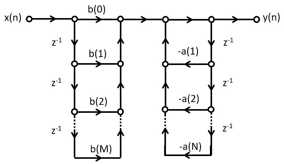
A direct-form I IIR implementation first computes the zeroes, and then the poles:

$Y(z) &= \frac{1}{A(z)}.[B(z).X(z)]$

In the time domain we would implement

$w(n) &= \sum_{k=0}^{M} b[k] x[n-k] \\ y(n) &= w(n) - \sum_{k=1}^{N} a[l] y[n-l]$

This formulation leads to a design as shown below. This design requires $1 + M + N$ multiplications per output sample, $M + N$ additions per output sample, and $M + N$ delays.

Direct-form II IIR Implementation 

A direct-form II IIR implementation first computes the poles, and then the zeroes:

$Y(z) &= B(z) . [\frac{1}{A(z)}.X(z)]$

This structure is created by swapping the order of the operations in a direct-form I structure. However, an important optimization is possible because the taps can be shared by the feedback part as well as by the feedforward part.

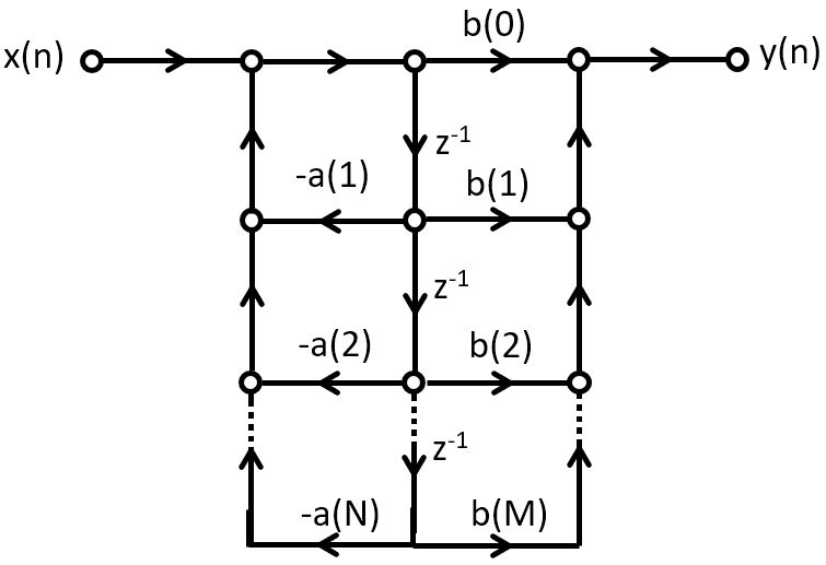
This design requires $1 + M + N$ multiplications per output sample, $M + N$ additions per output sample, and $max(M,N)$ delays.

This implementation has the mimimum number of delays possible for a given transfer function. Hence, an N-th order FIR, and an N-th order IIR, both can be implemented with only N delays.

Cascade IIR Implementation 

Just as with the FIR implementation, a cascade IIR is created by factoring the nominator and denominator polynomials in $G(z)$ . Assuming both nominator and denominator have order N, then

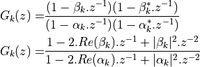
$G(z) =& \frac{\sum_{k=0}^{N} b[k] z^{-k}}{ 1 + \sum_{k=1}^{N} a[k] z^{-k}} \\ =& A . \prod_{k=1}^{N} \frac{1 - \beta_k . z^{-1}}{1 - \alpha_k . z^{-1}}$

It’s common to formulate this as second-order sections, in order to ensure that complex (conjugate) poles and complex (conjugate) zeroes can be represented with real coefficients. Each such a section contains a conjugate pole pair and/or conjugate zero pair.

$G_k(z) =& \frac{(1 - \beta_k . z^{-1})(1 - \beta_k^* . z^{-1})}{(1 - \alpha_k . z^{-1})(1 - \alpha_k^* . z^{-1})} \\ G_k(z) =& \frac{1 - 2.Re(\beta_k).z^{-1} + |\beta_k|^2.z^{-2}}{1 - 2.Re(\alpha_k).z^{-1} + |\alpha_k|^2.z^{-2}}$

Cascade IIR Example 

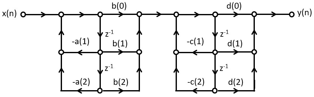
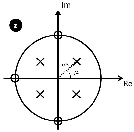
We implement the following cascade IIR design in C. It has four poles, located at $\pm 0.5 . e^{\pm j \pi/4}$ , as well as three zeroes, located at $j, -1, -j$ .

The first step is to derive the proper filter coefficients. We group the poles and zeroes as follows.

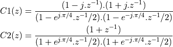
$C1(z) &= \frac{(1 - j.z^{-1}).(1 + j.z^{-1})}{(1 - e^{j.\pi/4}.z^{-1}/2).(1 - e^{-j.\pi/4}.z^{-1}/2)} \\ C2(z) &= \frac{(1 + z^{-1})}{(1 + e^{j.\pi/4}.z^{-1}/2).(1 + e^{-j.\pi/4}.z^{-1}/2)}$

Which can be multiplied out to derive the filter coefficients:

$C1(z) &= \frac{(1 + z^{-2})}{ (1 - \frac{1}{\sqrt 2}.z^{-1} + \frac{1}{4}.z^{-2})} \\ C2(z) &= \frac{(1 + z^{-1})}{ (1 + \frac{1}{\sqrt 2}.z^{-1} + \frac{1}{4}.z^{-2})}$

The construction of the filter proceeds similar to the cascade FIR filter. First, we create a data structure for the cascade IIR stage, containing filter coefficients and filter state. We will use a direct-form Type II design, which gives us a state of only two variables.

typedef struct cascadestate {
    float32_t s[2];   // state
    float32_t b[3];  // nominator coeff  b0 b1 b2
    float32_t a[2];  // denominator coeff   a1 a2
} cascadestate_t;

float32_t cascadeiir(float32_t x, cascadestate_t *p) {
    float32_t v = x - (p->s[0] * p->a[0]) -  (p->s[1] * p->a[1]);
    float32_t y = (v * p->b[0]) + (p->s[0] * p->b[1]) + (p->s[1] * p->b[2]);
    p->s[1] = p->s[0];
    p->s[0] = v;
    return y;
}

void createcascade(float32_t b0,
                   float32_t b1,
                   float32_t b2,
                   float32_t a1,
                   float32_t a2,
                   cascadestate_t *p) {
    p->b[0] = b0;
    p->b[1] = b1;
    p->b[2] = b2;
    p->a[0] = a1;
    p->a[1] = a2;
    p->s[0] = p->s[1] = 0.0f;
}

The cascadestate_t now contains both feed-forward and feed-back coefficients. The cascadeiir function is likely the most complicated element for this design. The order of evaluation of each expression is chosen so that we don’t update filter state until it has been used for all expressions required. In cascadeiir we first compute the intermediate variable v which corresponds to the center-tap of the filter. Next, we compute the feed-forward part based in this intermediate v. Finally, we update the filter state and return the filter output y.

The filter program then consists of filter initialization, followed by the chaining of filter cascades:

cascadestate_t stage1;
cascadestate_t stage2;

void initcascade() {
    createcascade(  /* b0 */  1.0f,
                    /* b1 */  0.0f,
                    /* b2 */  1.0f,
                    /* a1 */ -0.7071f,
                    /* a2 */ 0.25f,
                    &stage1);
    createcascade(  /* b0 */  1.0f,
                    /* b1 */  1.0f,
                    /* b2 */  0.0f,
                    /* a1 */ +0.7071f,
                    /* a2 */ 0.25f,
                    &stage2);
}

uint16_t processCascade(uint16_t x) {

    float32_t input = xlaudio_adc14_to_f32(0x1800 + rand() % 0x1000);
    float32_t v;

    v = cascadeiir(input, &stage1);
    v = cascadeiir(v, &stage2);

    return xlaudio_f32_to_dac14(v*0.125);
}

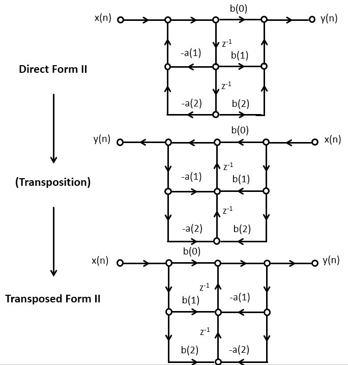
Transposed Structures 

The transposition theorem says that the input-output properties of a network remain unchanged after the following sequence of transformations:

Reverse the direction of all branches
Change branch points into summing nodes and summing nodes into branch points
Interchange the input and output

Once you have the defined the transposed-form structure, you can develop a C program for that implementation. The transposed-form IIR can be implemented using the same data structure as the direct-form IIR; only the filter operation would be rewritten. The following is the implementation of a second-order section of a transposed direct-form II design.

typedef struct cascadestate {
    float32_t s[2];   // state
    float32_t b[3];  // nominator coeff  b0 b1 b2
    float32_t a[2];  // denominator coeff   a1 a2
} cascadestate_t;

float32_t cascadeiir_transpose(float32_t x, cascadestate_t *p) {
    float32_t y = (x * p->b[0]) + p->s[0];
    p->s[0]     = (x * p->b[1]) - (y * p->a[0]) + p->s[1];
    p->s[1]     = (x * p->b[2]) - (y * p->a[1]);
    return y;
}

Parallel Structures 

IIR filters are rarely implemented as single, monolithic structures; the risk for instability is too high. One way to achieve this, is to use a cascade expansion of an IIR filter.

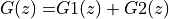
An alternate implementation is the parallel-form implementation. The idea of a parallel-from implementation is to build two or more parallel filters, that can be summed up together to form the overall transfer function.

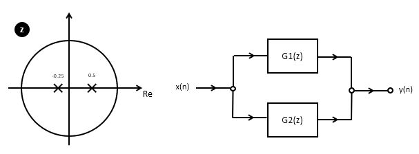
Let’s consider this for the pole plot shown in the figure. This design has two poles, so it’s transfer function would be:

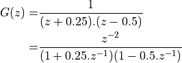
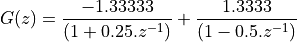
$G(z) =& \frac{1}{(z + 0.25).(z - 0.5)} \\ =& \frac{z^{-2}}{(1 + 0.25.z^{-1})(1 - 0.5.z^{-1})}$

To build a parallel design, we have to decompose $G(z)$

$G(z) =& G1(z) + G2(z)$

The design of these partial function proceeds by partial fraction expansion. We split the poles of the overall function $G(z)$ in two. In this case, one pole goes with $G1(z)$ and the other pole goes with $G2(z)$ . Partial fraction expansion will now proceed by looking for terms A and B such that:

$\frac{A}{(1 + 0.25.z^{-1})} + \frac{B}{(1 - 0.5.z^{-1})} = \frac{z^{-2}}{(1 + 0.25.z^{-1})(1 - 0.5.z^{-1})}$

Solving for A and B we find:

$G(z) &= \frac{-1.33333}{(1 + 0.25.z^{-1})} + \frac{1.3333}{(1 - 0.5.z^{-1})}$

The meaning of 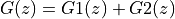$G(z) = G1(z) + G2(z)$ is that a second order system can be implemented by two independent first-order systems, whose output is added together.

Using Matlab 

In the following, we illustrate a few useful Matlab functions that help with the analysis and decomposition of IIR filters.

Finding Poles and Zeroes 

Attention

To identify pole and zero locations, use the roots function in Matlab, which finds the roots of a polynomial. For a polynomial $P(z) = a_0 + a_1 . z^{-1} + ... + a_n . z^{-n}$ , the roots can be found through roots([a0 a1 ... an])

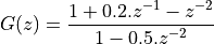
Example: Find the zeroes and poles of

$G(z) = \frac{1 + 0.2 . z^{-1} - z^{-2}}{ 1 - 0.5 . z^{-2}}$

The roots function in Matlab will return the locations of zeroes and poles:

>> roots([1 0.2 -1])  % numerator coefficients

ans =

   -1.1050
    0.9050

>> roots([1 0 -0.5])  % denominator coefficients

ans =

    0.7071
   -0.7071

>> zplane([1 0.2 -1],[1 0 -0.5])  % create a pole-zero plot

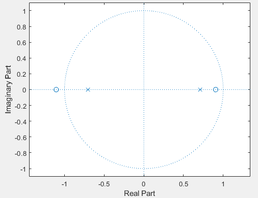
We can write G(z) in factored form as follows

$G(z) =& \frac{(1 - n_0 . z^{-1})(1 - n_1 . z^{-1})}{(1 - p_0 . z^{-1})(1 - p_1 . z^{-1}])} \\ G(z) =& \frac{(1 + 1.1050.z^{-1})(1 - 0.9050.z^{-1})}{(1 + 0.7071.z^{-1})(1 - 0.7071.z^{-1})}$

Finding Partial Fraction Expensions 

Attention

To perform partial fraction expansion, use the residue function in Matlab. For a transfer function 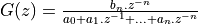$G(z) = \frac{b_n.z^{-n}}{a_0 + a_1.z^{-1} + ... + a_n.z^{-n}}$ the partial fraction is found as [r,p,k] = residue([0 0 ... bn], [a0 a1 .. an]).

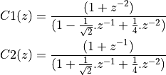
The parallel form of an IIR requires partial fraction expansion. Consider the following example, where the objective is to find A and B:

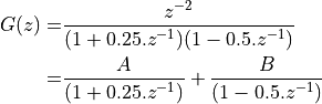
$G(z) =& \frac{z^{-2}}{(1 + 0.25.z^{-1})(1 - 0.5.z^{-1})} \\ =& \frac{A}{(1 + 0.25.z^{-1})} + \frac{B}{(1 - 0.5.z^{-1})}$

>> % compute G(z)
>> a = conv([1 0.25],[1 -0.5])

a =

   1.0000   -0.2500   -0.1250

% In other words, G(z) = z^-2 / (1 - 0.25.z^-1 - 0.125.z^-2)

>> % compute terms A and B using 'residue'
>> [r,p,k] = residue([0 0 1],a)

r =

    1.3333
   -1.3333

p =

    0.5000
   -0.2500

k =

     []

From the r term in the Matlab output, we conclude that

$G(z) &= \frac{-1.33333}{(1 + 0.25.z^{-1})} + \frac{1.3333}{(1 - 0.5.z^{-1})}$

Conclusions 

We discussed the following filter implementation techniques:

Direct Form I filters

Direct Form II filters

Transposed Direct Form II filters

We also discussed two decomposition techniques:

Cascade-form decomposition

Parallel-form decomposition