Real-time DSP Knowledge Domains 

Important

The purpose of this lecture is as follows.

To introduce the four knowledge domains that make up Digital Signal Processing implementations
To demonstrate how DSP design works through the design of a digital signal generator

When is it better to process signals digitally?

Let’s start this course by looking at the reasons why you’d use a computer to processor analog, physical quantities. Why not do everything in the analog, continuous-time domain? Analog processing is often much easier, less costly, and especially less power hungry than a fully digital solution. Compare, for example, (a) an analog low-pass filter built with a resistor and a capacitor to (b) a digital first-order low-pass filter.

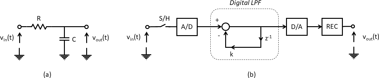
Clearly, the digital filter is more complex than the analog filter. To process signals digitally, you have to first convert the signal to a digital code using an analog-to-digital converter; then you have to process this discrete-time signal with a digital filter that approximates the analog filter, then you have to convert the digital code back to an analog continuous-time signal using a digital-to-analog converter, and finally you have to reconstruct the full analog signal by interpolating analog values in between the discrete samples of the digital filter. We will discuss the elements that make up a digital filter implementation in the coming lectures. But for now, let’s just ponder if we can identify arguments that make the digital filter design preferable over the analog design.

There are four arguments in favor of digital (over analog) signal processing.

No Loss of Precision: While the accuracy of digital computations is limited, digital computations are always exact. Computing twice the same output for the same input is a piece of cake in digital filter design. This robustness finds its origin in the discretization of continuous-value signals into bits - which can be implemented as high or low values with a noise margin. In contrast, analog signal processing does not enjoy the same margins, and noise will prevent exactly the same output from appearing under the same input. Analog components are also affected by environmental changes, as well as aging effects, and this directly affects their output as well.
No Tuning: Digital filters are built using discrete computations with constants. Once the constants are fixed, the digital filter is fully defined. In contrast, analog filters are created using components that may require period adjustment, and that have limited precision. Analog filter designs require tuning, while digital filters can be programmed as a series of constants.
Flexible: Digital signal processing implementations can be easily changed by chanfing of the filter constants. Furthermore, digital signal processing implementations can run on programmable platforms. For both of these reasons, digital signal processing implementations are naturally flexible. This is in constrast to analog filters built from discrete, fixed components.
Compatible with the Digital World: Finally, digital signal processing works with signals that are captured in the language of the internet, as discrete symbols that can be easily stored and transmitted. The bulk of data of interest today exists in digital form, and many applications of DSP live completely in the digital world.

The knowledge domains of Digital Signal Processing 

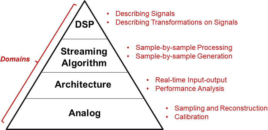
Digital Signal Processing implementations combine four knowledge domains.

Digital Signal Processing: The top DSP layer describes signals, and transformations on those signals. In DSP, signals are discrete-time, and the transformations on such discrete-time signals are described in discrete time steps.
Streaming Layer: The discrete-time signals in DSP are part of an infinite stream of signal samples, and each new sample in that stream comes at a regular interval called the sample rate. The sample rate defines the real-time character of Digital Signal Processing, as the processing will have to run as fast as new inputs become available. In the streaming layer, a DSP algorithm is expressed in such a manner that it can iteratively process this infinite stream of inputs.
Architecture Layer: This layer introduces resource contraints such as memory, digital logic, processors. The resource constraints have to be balanced against the amount of real-time processing that is required to implement the DSP algorithm as a streaming algorithm. Design in the architecture layer involves designing hardware or software.
Analog Layer: The bottom layer associates digital codes and numbers (integers, floating-point numbers, ..) with physical voltages according to a given calibrated scale. The analog layer also deals with analog-to-digital and digital-to-analog conversion.

A working DSP implementation does not involve just a single layer - but rather all of them. Each layer comes with its own challenges, be it digital filter design, digital filter implementation, coding in hardware or software, or signal sampling. In this course, we will spend most of our effort on DSP design for the streaming layer and the architecture layer.

An Example: Designing a DTMF generator 

As an illustration of each of the four layers discussed above (DSP, Streaming, Architecture, Analog), we’ll discuss the design of a touch-tone signal generator (or DTMF: Dual Tune Multi Frequency). DTMF codes are used by touch-tone telephones to encoded the keys of the telephone keypad.

First, what is DTMF? When you pick up an old touch-tone telephone and you press one of the number keys, you’ll here a characteristic tone for each key. It’s actually the combination of two tones. One tone encodes the keyboard row and the other tone encodes the keyboard column. The following table demonstrates the encoding of keys to frequencies. For example, key number ‘9’ is encoded as the sum of a 1477 Hz sine wave and a 852 Hz sine wave. The idea of DTMF is to support in-band signalling, which means that the voice band communication channel for telephone is use to relay control information (in the form of key presses). DTMF signalling involves both the generation of DTMF signals, as well as their detection. In this example, we will only worry about DTMF generation. However, it’s good to know that the DTMF standard specifies that a tone duration of 50ms should be sufficient to complete the detection of the key press.

DTMF standard frequencies
Freq (Hz)	1209	1336	1477	1633
697	Key ‘1’	Key ‘2’	Key ‘3’	Key ‘A’
770	Key ‘4’	Key ‘5’	Key ‘6’	Key ‘B’
852	Key ‘7’	Key ‘8’	Key ‘9’	Key ‘C’
941	Key ‘*’	Key ‘0’	Key ‘#’	Key ‘D’

DTMF Generator: DSP Layer 

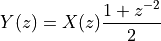
The highest level specification of a DTMF generator is purely algorithmic. We could just describe a DTMF signal as a math equation as a function of time.

$y(t) = sin(2 \pi f_R t) + sin(2 \pi f_C t)$

In this equation, $f_R$ and $f_C$ represent the row and column frequency, respectively. This representation is nice and compact from a mathematical perspective, but it doesn’t capture the inputs of the DTMF Generator very well. Indeed, time is an independent variable in this equation, it’s not really an input to the DTMF generator. Rather, the input consists of the two variables $f_R$ and $f_C$ .

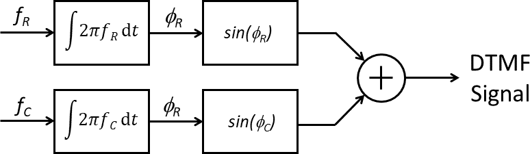
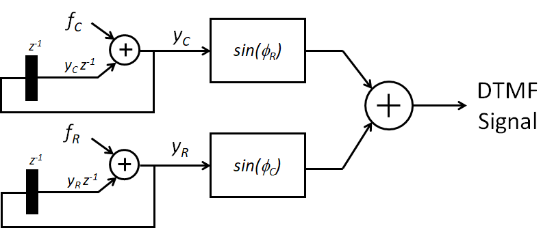
In DSP, it’s common to describe systems as a block diagram. Each of the blocks is a simple function, that accepts one or more inputs. For example, here is a block diagram of a DTMF generator. Given two constant $f_R$ and $f_C$ , we first compute $2 \pi f_R t$ and $2 \pi f_C t$ , which represent the phase of row and column since wave, respectively. Note that time is not used as an input in this block diagram; time is a universal indepent variable for everything, and we can only express changes of other variables as a function of time. For this reason, the block diagram introduces two integrator blocks, which take a frequency, and convert it to a phase by integrating the frequency value over time.

The block diagram shown above is expressed using continuous time, while DSP systems use discrete-time, meaning that time advances in discrete time steps. The period of these steps is called the sample period, and its reciprocal is called the sample frequency. A common choice for DTMF signals is a sample frequency of 8 KHz, which is what is commonly used for voice-band signals.

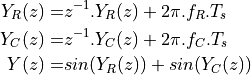
The discrete-time representation of an integral is an accumulation (sum) of discrete-time quantities. Each sample period, the phase of $\phi_R$ and $\phi_C$ increase an a small amount, $2\pi.f_R.T_s$ and $2\pi.f_C.T_s$ respectively. This allows to write the continuous-time integrals as recurrence equations, and the complete DTMF generator becomes a discrete-time algorithm.

$y_R[n] =& y_R[n-1] + 2\pi.f_R.T_s \\ y_C[n] =& y_C[n-1] + 2\pi.f_C.T_s \\ y[n] =& sin(y_R[n]) + sin(y_C[n])$

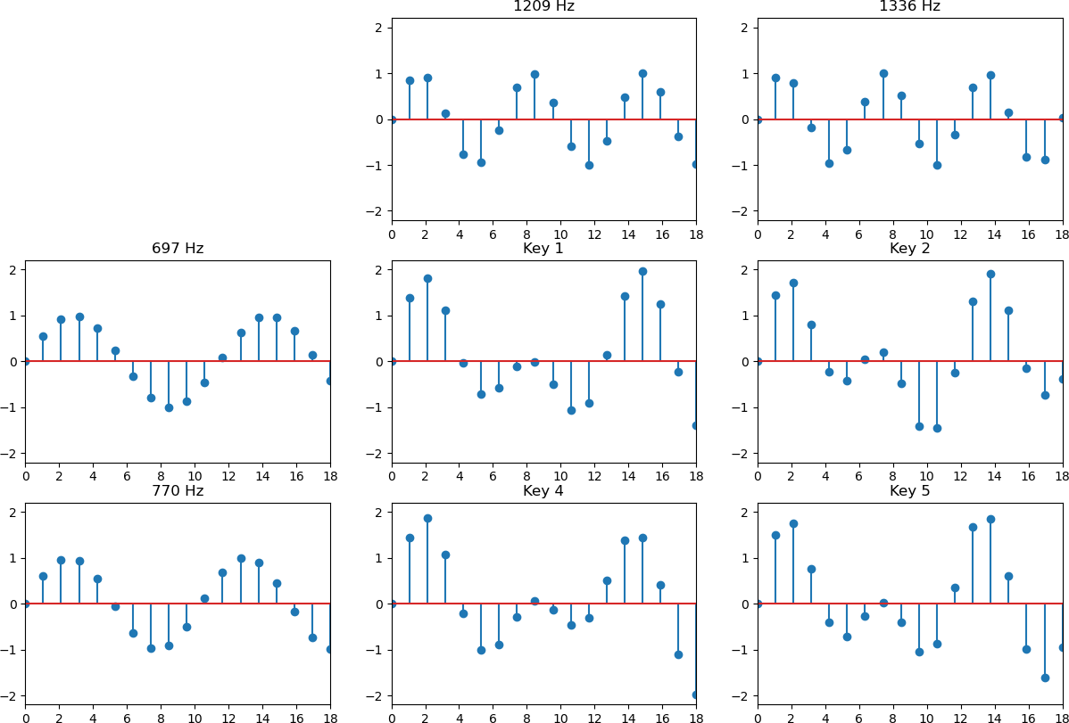
We will elaborate in further detail on this transition from continuous-time to discrete-time in a future lecture. For now, we’ll just work with these recurrence equations. Using the recurrence equations, we can now see how the DTMF generator works, for example in Matlab. Simple compute the output y[n] for several periods of a row/column sine wave helps you visualize the shape of a DTMF signal. Here is an example for the keys 1, 2, 4 and 5.

DTMF Generator: Streaming Layer 

The second layer of the DSP pyramid is the streaming layer. There are two important concepts that are introduce at this layer: the time loop, and the algorithm state. The time loop introduces time explicitly in the computation of the DSP output. Indeed, a recurrence relation by itself (e.g. $y[n] = y[n-1] + 1$ ) does not imply time; time is only introduced by explicitly associating the dimension of the recurrence equation with the time axis. In this context, $y[n]$ stands for ‘the current output’, and $y[n-1]$ stands for ‘the previous output’. Similarly, consider the following recurrence equation.

$y[n] = \frac{x[n] + x[n-2]}{2}$

In this context, $y[n]$ stands for the current output, $x[n]$ stands for the current input, and $x[n-2]$ stands for the previous previous input.

Imagine that the input signal $x$ is an infinite stream of input samples, spaced in time by a sample period, and that the output signal $y$ is an infinite stream of output samples, spaced by the same sample period.

The time loop expressed the recurring activities that happen to compute the current output, given the value of the previous output(s) and the current and previous input(s).

The second concept, DSP algorithm state, is a consequence of creating the time loop. In order to access a previous input or output, we have to store the current input or output one or more samples. These storage locations are often referred to as ‘delays’. We use the Z-transform to conveniently express these delays. In particular, by representing the Z-transform of $x[n]$ as $X(z)$ , we can capture the Z-transform of $x[n-1]$ as $z^{-1}.X(z)$ . So the previous equation can be written as follows.

$Y(z) = X(z) \frac{1 + z^{-2}}{2}$

We will elaborate on the Z-transform in a later lecture. For now, the association of $z^{-1}$ as a delay of a single sample is sufficient. The DTMF recurrence equations can be mapped to a time loop as follows. First, determine the Z-transform of the DTMF generator.

$Y_R(z) =& z^{-1}.Y_R(z) + 2\pi.f_R.T_s \\ Y_C(z) =& z^{-1}.Y_C(z) + 2\pi.f_C.T_s \\ Y(z) =& sin(Y_R(z)) + sin(Y_C(z))$

Next, prepare a diagram to visualize the operation. The generation of a sine signal thus has two state variables, one for each of the phases of row and column frequency, respectively.

It’s also convenient to express the timeloop in pseudocode, since that can serve as a blueprint for a software program that generates the DTMF signal. The following pseudocode program demonstrates this idea. Of course, you have to keep in mind that there is an implicit assumption made regarding the real-time behavior, namely that the loop will complete one iteration per sample period.

statevar old_yr;
statevar old_yc;

/* DTMF time loop */
repeat forever {

   read input fr;
   read input fc;

   yr = old_yr + fr;
   yc = old_yc + fc;
   q  = sin(yr) + sin(yc);

   write output q;

   old_yr = yr;
   old_yc = yc;
}

DTMF Generator: Architecture Layer 

The third layer of design of a Real Time Digital Signal Processing system is the architecture layer. They key objective of this layer is to map a streaming algorithm to a limited set of computation resources. In the architecture layer, we figure out how to deal with resource constraints of the implementation. In this course, we will implement streaming algorithms in software. The resource constraints of software implementations include the limited processing speed of the microprocessor to run the DSP program, the limited program and data memory available to store the DSP program and its intermediate variables, and the limited precision of the computations performed by the microprocessor. Dealing with resource constraints is not easy and requires design practice; a considerable portion of the course work will be spent on implementation aspects of Real-time DSP.

Writing real-time C code 

We can take the time loop implementation of the DTMF generator developed earlier, and write it as a C program. However, an important challenge is that the C program has to run in real time. Real-time execution, in the context of a DSP program, does not mean: execute as fast as possible. Instead, real-time execution means: execute as fast as needed. The time-loop is designed to run at the sample period of the input sample stream. For each iteration of the time-loop, a single input is read (the input sample), and a single output is writtten (the output sample).

Now, imagine that the DTMF generator is written as a function with a single input and a single output. The problem of real-time execution now is, that we have to guarantee that the function is called once at each sample period. Of course, the underlying assumption is that the function call itself will finish in a time shorter than each sample period. One solution to this real-time execution problem, is to use a so-called periodic interrupt. A hardware timer is used to count periods that are as long as a the sample period. Every time the hardware timer expires, it generates an interrupt to a microprocessor that contains the DSP time loop function. And the interrupt service routine itself kicks off the execution of the DSP function. This way, we are able to guarantee the input and output sample rate of the DSP processor, even if we don’t know precisely how long the DSP processing itself takes.

Writing DTMF Generation in C 

Next, we have to create the sine function required for the DTMF generator. We’ll show how this can be done using integer computations on a lookup table. Since we are only interested in a limited number of frequencies, we will precompute the sine values that are needed to compute each row and column frequency of interest.

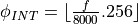
The tables are computed as follows. The samples are generated at 8000 Hz. A given DTMF frequency, say 697 Hz, can be expressed as a fraction of the sample frequency. The resulting fractional number $\phi$ , between 0 and 1, represents the fraction of the circle traveled by the phase of the DTMF frequency during one sample period.

That fractional number can then be scaled up to an integer value $\phi_{INT}$ with a given resolution. The integer phase range determines the number of entries required in a lookup table holding sine values. The following table shows that the integer phase step for 697 Hz equals 22, for a scale-up factor of 256. Given a sine table with 256 entries, the 697 Hz frequency can be approximated at 8 KHz by successively returning entry 22, 44, 66, 88, .., n.22 mod 256. Because the phase step is quantized, there is a small error of the generated frequency when compared to the targeted DTMF frequency. The table shows that, at 8 bit phase resolution, the maximum frequency error is below 10 Hz for any DTMF frequency.

DTMF phase step computation
f (Hz)	$\phi = \frac{f}{8000}$	$\phi_{INT} = \lfloor \frac{f}{8000}.256 \rfloor$	$f_{actual}$ (Hz)	Error (Hz)
697	0.087125	22	687.5	9.5
770	0.09625	25	781.25	-11.25
852	0.1065	27	843.75	8.25
941	0.117625	30	937.5	3.5
1209	0.151125	39	1218.75	-9.75
1336	0.167	43	1343.75	-7.75
1447	0.184625	47	1468.75	8.25
1633	0.204125	52	1625	8

A second implementation challenge is that of the resolution of the sine implementation. In the DTMF implementation, we will compute the sine on 16-bit precision, namely using the integer values $-2^{15} .. 2^{15}-1$ , or -32768 to 32767. Combined with the phase generation concept described earlier, the sine values can thus be stored in a table of 256 entries (corresponding to the phases) with each entry a 16-bit integer number (corresponding to the sine values). In addition, because of the symmetry in the sine function, we only need to store one quarter of the wave form.

dtmf.c

// Quantized sine value table generated using python:
//
// import numpy
// for i in xrange(64):
//   print(numpy.sin(i / 64 * numpy.pi / 2)*32767)

int sinelookup[64] = {
    0,  804, 1607, 2410, 3211, 4011, 4807, 5601,
 6392, 7179, 7961, 8739, 9511,10278,11038,11792,
12539,13278,14009,14732,15446,16150,16845,17530,
18204,18867,19519,20159,20787,21402,22004,22594,
23169,23731,24278,24811,25329,25831,26318,26789,
27244,27683,28105,28510,28897,29268,29621,29955,
30272,30571,30851,31113,31356,31580,31785,31970,
32137,32284,32412,32520,32609,32678,32727,32757};

int rowinc[4] = { 22, 25, 27, 30};
int colinc[4] = { 39, 43, 47, 52};

int qmapsine(int f) {
   if (f < 64)
      return sinelookup[f];
   else if ((f - 64) < 64)
      return sinelookup[127 - f];
   else if ((f - 128) <  64)
      return -sinelookup[f - 128];
   else
      return -sinelookup[255 - f];
}

int outputsample(int row, int col) {
   static int rowphase = 0;
   static int colphase = 0;

   rowphase = (rowphase + rowinc[row & 3]) & 255;
   colphase = (colphase + colinc[col & 3]) & 255;

   return qmapsine(rowphase) + qmapsine(colphase);
}

DTMF Generator: Analog Layer 

The bottom layer of the DSP pyramid is the Analog Layer, which governs the mapping of analog voltage levels to digital values and back. The conversion of analog voltages to digital values is done using an analog-to-digital converter, while the opposite conversion is done using a digital-to-analog converter.

Let’s design the D/A code generation for the DTMF generator. The generator creates a waveform with a 16-bit amplitude, and discrete waveform points are captured as integers between -32768 and 32767. A D/A converter is attached to the microprocessor over a standard bus. However, the D/A converter may not have the same resolution as the program.

In this example, we demonstrate how to scale the 16-bit output of C for a 14-bit D/A converter. We assume that the 14-bit D/A converts the output codes 0 to $2^{14} - 1$ to the output voltages 0 volt to 2 volt. Also, we aim to create a DTMF output signal that does not exceed 500mV peak-to-peak around a constant offset. The question then is to define the correct scaling formula to transform the 16-bit values computed in C into 14-bit output codes that generate the proper waveform.

The following figure graphically demonstrates this conversion. On the left side, the C program creates values between -32768 and 32767. On the right side. The D/A converter accepts codes between 0 and 16383.

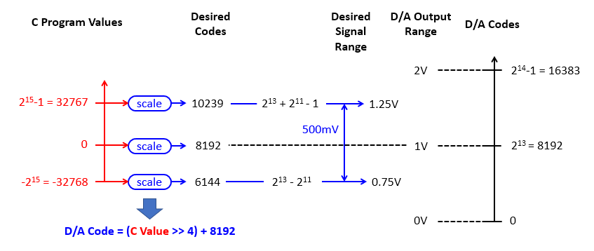
_images/dacalibrate.png — This image shows how a 16-bit value can be mapped into a 500mVpp range on a 14-bit D/A converter. The calibration involves identifying the output codes corresponding to the desired voltage range, and next creating a scaling formula to convert 16-bit C values to 14-bit D/A codes with the desired range.

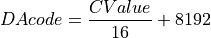
The range of codes that limits the output to a 500mV peak-to-peak waveform likes between one quarter and three quarters of the D/A code range, which corresponds to the codes 6144 to 10239. The ground-level value, corresponding to 0 in the C program, maps to D/A code 8192, which is the midpoint (1 Volt). This settles the conversion from C output values to D/A codes with the following conversion formula.

$DAcode = \frac{CValue}{16} + 8192$

DTMF Generator: Bringing it all together 

We have developed the major parts of the DTMF Generator; the final remaining step is to map it on a practical platform. We will be using an MSP-EXP432P401R Launchpad and a AUDIO-BOOSTXL analog front-end. The specifications of this hardware are described in detail in the Data Sheets and User Guides.

The major missing element is the real-time input/output aspect. To help you write real-time DSP programs, we will use a library that was written specifically for this course. The library XLAUDIO_LIB provides a basic programmer’s interface (API) to write DSP code. In the following, we’ll dive straight into the programming of DTMF signal generation on our DSP platform. The following listing contains the complete DTMF generator.

dtmfmsp.c

#include "xlaudio.h"
#include <ti/devices/msp432p4xx/driverlib/driverlib.h>
#include "xlaudio_armdsp.h"

int sinelookup[64] = {
      0,  804, 1607, 2410, 3211, 4011, 4807, 5601,
   6392, 7179, 7961, 8739, 9511,10278,11038,11792,
  12539,13278,14009,14732,15446,16150,16845,17530,
  18204,18867,19519,20159,20787,21402,22004,22594,
  23169,23731,24278,24811,25329,25831,26318,26789,
  27244,27683,28105,28510,28897,29268,29621,29955,
  30272,30571,30851,31113,31356,31580,31785,31970,
  32137,32284,32412,32520,32609,32678,32727,32757};

int rowinc[4] = { 22, 25, 27, 30};
int colinc[4] = { 39, 43, 47, 52};

int qmapsine(int f) {
   if (f < 64)
      return sinelookup[f];
   else if ((f - 64) < 64)
      return sinelookup[127 - f];
   else if ((f - 128) <  64)
      return -sinelookup[f - 128];
   else
      return -sinelookup[255 - f];
}

int outputsample(int row, int col) {
   static int rowphase = 0;
   static int colphase = 0;
   rowphase = (rowphase + rowinc[row & 3]) & 255;
   colphase = (colphase + colinc[col & 3]) & 255;

   return qmapsine(rowphase) + qmapsine(colphase);
}

int dtmfcode = 0;
typedef enum {IDLE, INC, DEC} audiostate_t;

audiostate_t next_state(audiostate_t current) {
    audiostate_t next;

    next = current;    // by default, maintain the state

    switch (current) {
    case IDLE:
        if (xlaudio_pushButtonLeftDown()) {
            next = INC;
            dtmfcode = (dtmfcode + 1) % 16;
            printf("%d\n", dtmfcode);
        }
        else if (xlaudio_pushButtonRightDown()) {
            next = DEC;
            dtmfcode = (dtmfcode + 15) % 16;
            printf("%d\n", dtmfcode);
        }
        break;

    case INC:
        if (xlaudio_pushButtonLeftUp())
            next = IDLE;
        break;

    case DEC:
        if (xlaudio_pushButtonRightUp())
            next = IDLE;
        break;

    default:
        next = IDLE;
    }

return next;
}

audiostate_t glbAudioState = IDLE;

uint16_t processSample(uint16_t x) {
    // the FSM controls the value of dtmfcode (0 .. 15)
    glbAudioState = next_state(glbAudioState);

    // the DTMF generator converts the code to a sine sample
    int q = outputsample(dtmfcode / 4, dtmfcode % 4);

    // the DTMF sample is mapped to a 500mV peak-to-peak waveform
    return (8192 + q / 16);
}

#include <stdio.h>

int main(void) {
    WDT_A_hold(WDT_A_BASE);

    xlaudio_init_intr(FS_8000_HZ, XLAUDIO_MIC_IN, processSample);
    xlaudio_run();

    return 1;
}

dtmfmsp.c integrates the DTMF generator on the MSP432P401R microcontroller. The code is most easily understood by starting with the main function. Two function calls, xlaudio_init_intr and xlaudio_run, set the system up for real-time signal processing with a sample frequency of 8 KHz. Each 125 $\mu s$ ( $\frac{1}{8 KHz} = 125 \mu s$ ), the function processSample is called; we will discuss the mechanism of achieving the real-time character in a separate lecture. The function processSample uses a finite state machine, mapped in next_state, to determine the current DTMF tone that is to be generated. The variable dtmfcode will contain a number of 0 to 15 depending on what DTMF tone is to be created. Next, the function outputsample delivers the actual value of the DTMF tone at that instant. This function is taken directly from dtmf.c. Finally, the 16-bit output resolution of outputsample is scaled to the 14-bit precision of the DAC, and the sample is converted in audio. The complete execution of processSample must finish within 125 $\mu s$ to maintain real-time operation.

The purpose of the state machine in next_state is to determine what DTMF tone to generate. The state machine reads the state of the left and right button of the MSP-EXP432P401R board to increment resp. decrement the DTMF tone code. The state machine requires each button to be released before incrementing/decrementing the DTMF tone code again.

This Figure shows a snapshot of an oscilloscope monitoring the signal that is fed into the audio amplifier, when the program is generating the waveform for DTMF key ‘3’. The top half shows the time-domain signal captured from the MSP-EXP432P401R board. The bottom half shows the spectrum of the signal shown in the top half. There are two clear peaks marked, one at around 670Hz and the other at around 1460Hz. These frequencies mark the row and column respectively, of the DTMF code. The output signal also contains image frequencies at (8000-670)Hz and (8000-1460)Hz. These frequencies appear because the reconstruction capabilities of the BOOSTXL-AUDIO board are limited. The reconstruction filter on BOOSTXL-AUDIO is a first-order lowpass filter with a cutoff frequency of about 20KHz.

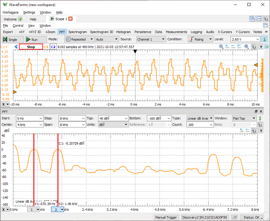
_images/mspdtmfcode.png — This figure shows the output of the DTMF code generator when creating the waveform for key ‘3’. The upper half shows the time-domain, the bottom half shows the frequency spectrum.