Lab 4: Quantization Effects in DSP

The purpose of this assignment is as follows.

to study the impact of quantization on a signal spectrum,
to study the impact of quantization on a filter characteristic,
to measure quantization noise by comparing a floating-point and a fixed-point filter in real time.

Fixed Point Implementation requires Quantization

In class, we discussed a technique to reduce the implementation cost (energy-wise or performance-wise) of a DSP design, by converting the floating-point computations to fixed-point computations. A side-effect of fixed-point design is the requirement to reduce the resolution (precision) of a signal representation. In a fixed-point representation of fix<N,k>, the weight of the least significant bit carries the fixed value $2^{-k}$ , and no changes smaller than that quantity can be represented.

We will study the consequences of the conversion from floating-point representation to fixed-point representation by means of a series of three experiments. For each experiment, you will have to write (or modify) a short program, run it on your board and analyze the resulting signal in the time domain or in the frequency domain. The outcome of this lab consists of the software programs you will write as specified, and the written report with the analysis of the effects you observe.

Impact of Quantization in the time and frequency domain

To support your experiments, you must first write two functions.

int float2q(float x, int f) {
   // .. written by you
}

float2q(x,f) converts a floating point number x to a fixed point number fix<32,f>. The output datatype is an int, a signed integer. The lecture notes explain the relation between floating point representation and fixed point representation.

float q2float(int q, int f) {
   // .. written by you
}

q2float(q,f) converts a fixed point number q of type fix<32,f> to a floating point number.

With these two functions in hand, we can study the effect of fixed-point refinement, that is, we can study the effect of quantization on a DSP program written with float. For example, to quantize the floating point number 0.1 to 5 fractional bits, we write:

float p = q2float(float2q(0.1, 5), 5);

In this example, p will be quantized to 0.09375, which is $2^{-4} + 2^{-5}$ , or the fractional bitpattern .00011.

Your first task is to write a program that passes the input to the output while quantizing the signal to k fractional bits. Then, you will apply a 500 Hz sinusoid to the input, and study the spectrum of the output signal with and without quantization. You can complete the program lab4_q1 to achieve the required implementation for this part.

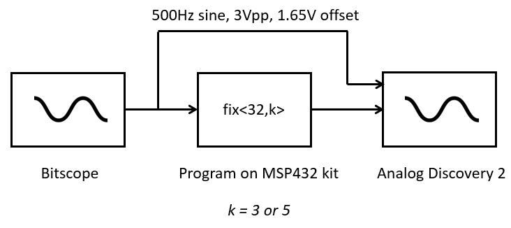
Once you have written the program, construct the setup as shown on the figure above. Using Analog Discovery 2 Scope, apply a 500Hz sine wave, 3V peak-to-peak, 1.65V offset to the ADC input. Capture the output of the DAC (after the lowpass reconstruction filter), and monitor both input and output on the oscilloscope.

Next, compare the following three designs.

The output is directly passed from the input:

output = input

The output is quantized on a fix<32,5>:

output = q2float(float2q(input, 5), 5);

The output is quantized on a fix<32,3>:

output = q2float(float2q(input, 3), 3);

Important

Question 1: For each implementation case described above, answer the following questions.

In the time domain, describe the waveform. Explain anomalies and non-linearities, and in particular try to explain the cause of anomalies and non-linearities.

In the frequency domain, describe the spectrum over the entire band from DC to the sampling frequency. Identify anomalies and try to explain their cause.

Finally, make sure to compare these three cases to each other (i.e., compare the case of no quantization, to quantization with 5 fractional bits, to quantization with 3 fractional bits). We are looking for more than just a single line of text; make a good analysis of what you see.

You can use the pushbutton functions of the xlaudio library for quick comparison of implementations. For example, you can write the processSample filtering function as follows.

uint16_t processSample(uint16_t x) {
  float input;

  input = adc14_to_f32(x);

  float v;
  if (pushButtonLeftDown()) {
    v = input;
  } else {
    v = q2float(float2q(input,5),5);
  }

  return f32_to_dac14(v);
}

This code will pass the input to the output, but will quantize the output to 5 fractional bits when you press the left button. This enables you to quickly compare the spectrum of the non-quantized case to the quantized case.

Impact of Quantization on filter characteristic

Next, we will study the impact of quantization on filter coefficients. Consider a first-order high-pass filter.

$H(z) = \frac{1}{1 - a.z^{-1}}$

This filter has a single pole at location $z = a$ (where $a$ is a negative number between -1 and 0). In a filter with quantized coefficients, the location of the poles (or zeroes) can shift compared to their original floating-point position. This, in turn, will affect the filter characteristic.

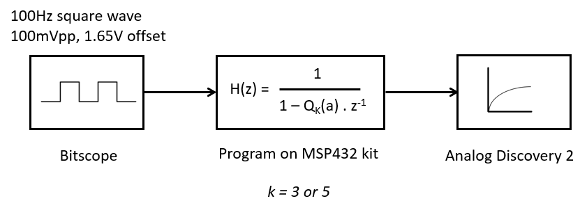
Now construct a program that implements a first-order low-pass filter, where ONLY the filter coefficient is quantized. You can do this with the same functions as used earlier, i.e. to quantize floating-point coefficient a with k fractional bits, use q2float(float2q(a,k),k). Implement the filter with a pole located at $z = -0.92$ . You can complete the program lab4_q2 to achieve the required implementation for this part.

Next, construct a measurement setup that applies a square wave at the input with 100 mV amplitude, 1.65V offset, and 100 Hz. Observe the output in the time domain, and compare three cases.

The filter coefficient a is unmodified
The filter coefficient a is quantized to k=5 fractional bits
The filter coefficient a is quantized to k=3 fractional bits

Important

Question 2: For each implementation case described above, precisely observe the output waveform in the time domain. Note the amplitude and offset of each output waveform. Are they identical or not? Explain the cause of your observations by your insight in the quantization process and its effect on the filter coefficient of $H(z)$ .

Measuring Quantization Noise of a Fixed-point Filter Design

The final part of the lab is to implement a complete filter as a fixed-point design. We will quantize the input and output, as well as the filter coefficients. Instead of doing floating-point computations, we will implement the entire filter using integer computations. We will measure the response of this quantized filter, and measure its quantization noise by comparing with a floating-point version of the same filter in real time.

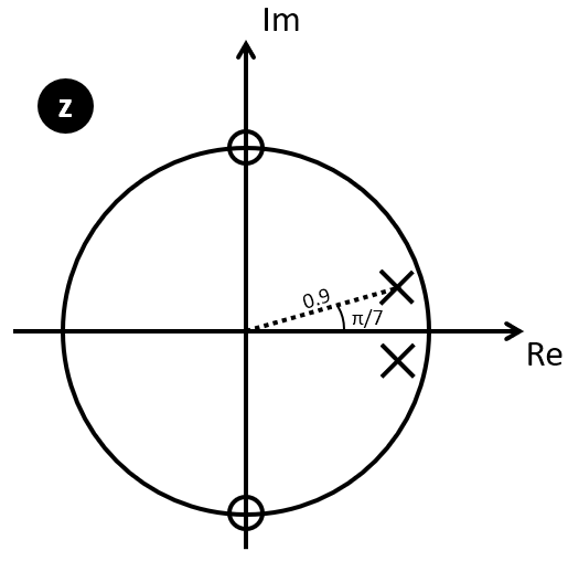
The filter you have to implement is a second-order filter described by the following pole-zero plot. The zeroes are located at $n_{1,2} = e^{\pm j \pi/2}$ and the poles are located at $p_{1,2} = 0.9 e^{\pm j \pi/7}$ .

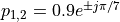In selecting the filter coefficients, pay attention to the proper scaling of filter coefficients. Ideally, the sum of the absolute filter coefficients should be equal to 1. For example, if you scale each filter coefficient $h_i$ by $\frac{1}{\sum_i (abs(h_i))}$ , the filter has unit power. This scaling helps to prevent overflow at the output.

Step 1: Floating Point Version in Matlab

Build a reference model for the filter in Matlab, with the same poles and zeroes. Obtain the impulse response of that filter. Don’t use filterDesigner, but use Matlab directly to compute the impulse response. This can be done easily through code as shown below.

b = conv([1 j], [1 -j]);
a = conv([1 -0.9*exp(-j * pi / 7)],[1 -0.9*exp(j * pi/7)]);
x = zeros(100,1);
x(20) = 1;           % add an impulse
figure(1)
plot(filter(b,a,x)); % plot the impulse response
figure(2)
freqz(b,a); % plot the spectrum and phase

Make a plot of the impulse response of the filter and keep that aside.

Step 2: Floating Point Version in C

Now, build a C version of this filter according to the following flow diagram.

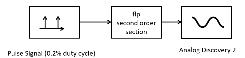
The second-order section can be implemented using an architecture of your choice: direct-form I or II, or transposed direct-form. Refer to the examples discussed in class for sample source code for such filters.

Design your filter for an 8 KHz sample rate. The input of the filter is a repetitive impulse with a 1/500 duty cycle (0.2%), which translates to a pulse frequency of 16 Hz. The very low duty cycle is there so you can observe the impulse response of the filter.

Pay attention in choosing the proper triggering settings for the oscilloscope. You have to sample an impulse response that happens 16 times per second, but you have to sample it at a sufficiently high sample rate, say 2 ms/Div on the scope. Thus you may need to add trigger delay in order to capture the signal in its entirety.

Important

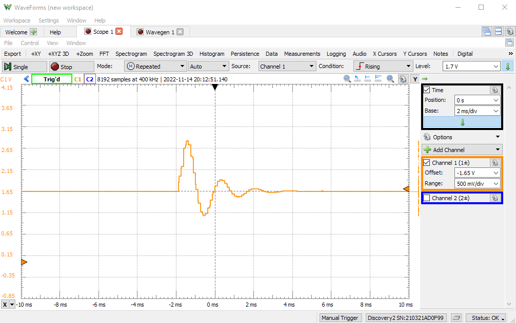
Question 3: Build the filter and capture its impulse response from the oscilloscope. Compare the impulse response to the impulse response computed in Matlab. They should look very similar, of course. Comment on any differences you detect, in the time domain as well as in the frequency domain.

You may do this comparison directly in Matlab, by recording the impulse response and importing the signal in Matlab.

Step 3: Fixed Point Version in C

Next, quantize the C version of this filter according to the following flow diagram.

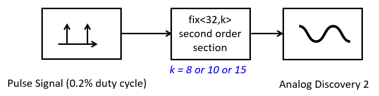
The fixed-point design will have to run a given fractional precision, programmable at 8 bits, 10 bits or 15 bits. Quantization applies to all aspects of the filter: the coefficients, the signals as well as to the intermediate results.

Your filter needs to support only one quantization level at a time. Thus, your code can use a macro PRECISION which you can set at 8, 10, or 15. You can recompile your code to change the quantization level.

To scale the output of the ADC to 8 or 10 bits, work as follows. Use a xlaudio_adc14_to_q15() function to convert an ADC code to fix<32,15>. Then scale the input to the proper precision by additional shifts. For example, to get an 8-bit output, use xlaudio_adc14_to_q15(...) >> (15 - 8). To quantize to a precision level of PRECISION bits, use xlaudio_adc14_to_q15(...) >> (15 - PRECISION).

You can use a similar conversion to scale the signal from PRECISION bits to 15 bits (Q15 precision) when you convert the signal to the DAC. Use xlaudio_q15_to_dac14(... << (15 - PRECISION)).

Refer to the example from class for guidance on writing a fixed-point precision filter. In essence, you have to rewrite the solution of Question 3 with fixed-point precision.

Important

Question 4: Build the filter and capture its impulse response from the oscilloscope for 8, 10 and 15 bits of precision. Compare the impulse response to the impulse response computed in Matlab. Comment on any differences you detect, in the time domain as well as in the frequency domain.

You may do this comparison directly in Matlab, by recording the impulse response and importing the signal in Matlab.

Wrapping Up

The answer to this lab consists of a written report which will be submitted on Canvas by the deadline. Refer to the General Lab Report Guidelines for details on report formatting. You will only submit your written report on Canvas. All code developed must be returned through GitHub.
Follow the principal structure of the report you’ve used for Lab 3 (taking into account any feedback you have received).
Follow the four questions outlined above to structure your report. Use figures, screenshots and code examples where appropriate. Please work out the answers in sufficient detail to show your analysis.
Make sure that you add newly developed projects to github: Use the Team - Share pop-up menu and select your repository for this lab. Further, make sure that you commit and push all changes to the github repository on GitHub classroom. Use the Team - Commit pop-up menu and push all changes.
Be aware that each of the laboratory assignments in ECE4703 will require a significant investment in time and preparation if you expect to have a working system by the assignment’s due date. This course is run in “open lab” mode where it is not expected that you will be able to complete the laboratory in the scheduled official lab time. It is in your best interest to plan ahead so that you can use the TA and instructor’s office hours most efficiently.

Good Luck

Grading Rubric

Requirement	Points
Question 1 Analysis	15
Question 2 Analysis	15
Question 3 Analysis	20
Question 4 Analysis	25
All projects build without errors or warnings	5
Code is well structured and commented	5
Git Repository is complete and up to date	5
Overall Report Quality (Format, Outline, Grammar)	10
TOTAL	100