Lab 6: BPSK Modulator

The purpose of this assignment is as follows.

to implement an optimized symbol shaping filter for BPSK modulation
to analyze the assembly code generated from the compiler-optimized implementation of the filter

BPSK Modulator

In this lab, we will implement a Binary Phase-Shift Keying (BPSK) modulator. We refer to the lecture of 5 December for the technical background on BPSK; in this lab, you will receive a complete filter design specification. You will have to design the filter using Matlab, and next create an optimized C code implementation. From the optimized C code implementation, we will then generate assembly code and analyze the cycle count of the implementation.

The following figure illustrates the overall design of the BPSK modulator.

A symbol stream of bits encoded as the symbols -1 and +1 is up-sampled to 8 samples per symbol. The upsampler inserts 7 zeroes for every symbol, so that the sample rate after the upsampler is 8 times higher then at the input of the upsampler. The resulting pulse stream contains +1 and -1 pulses with 7 zeroes in between each pulse.
This upsampled pulse stream is then filtered through a root-raised-cosine pulse-shaping filter, which is a finite impulse response filter (FIR) with a predefined shape. This particular filter is 6 symbols wide. At 8 samples per symbol, the filter contains 41 taps in total (5 x 8 taps + 1 center tap). The purpose of the filter is to shape the symbol pulse stream to a smooth, interpolated curve.
Finally, the pulse-shaped sample stream is up-converted using double side-band modulation to a carrier at one fourth of the sample frequency. Upconversion is implemented by multiplying with a cosine at the carrier frequency. Note that this particular carrier frequency, fs/4, yields cosine values of 1, 0, and -1 only.

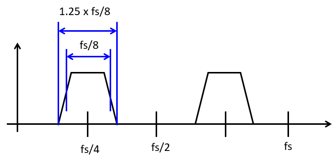
This BPSK modulation system can transmit bits at a rate of 1/8th of the sample rate, or fs/8, and uses a bandwidth of approximately ((1 + rolloff) . fs/8) = 1.25 . fs/8. The modulated signal uses a carrier of fs/4. The following figure shows the spectrum at the output of this BPSK modulator, assuming that it is transmitting a sequence of random symbols. You can see how this BPSK modulation system is useful: it can transmit bits at a rate of fs/8 while using a bandwidth just a little bit wider than the bitrate. For example, in a bandwidth of 1250 Hz, we can encode 1000 bits/second.

In the following steps, you will systematically develop this BSPK modulation system, check the bandwidth of the generated modulated signal, and eventually build a performance-optimized implementation of the design.

Step 1: Raised-cosine design

The first step is to develop a Matlab version of the modulator you will build in C. The following are a set of useful functions in Matlab to help you visualize the output.

% Generate a raised-cosine pulse with rolloff factor, rcsymbols wide, at samplespersymbol
rcp       = rcosdesign(rolloff, rcsymbols, samplespersymbol);

% Generate a stream of numsymbols random BPSK symbols (-1, +1)
symbols   = (floor((rand(numsymbols,1) * 2)) - 0.5) * 2;

% Create an upsampled signal from a symbol stream
upsampled = upsample(symbols, samplespersymbol);

% Filter the upsampled signal with the raised-cosine pulse shaper
rcupsym   = conv(upsampled, rcp);

% Generate a carrier signal at fs/4 over symbols at samplespersymbol
carrier   = cos(2 * pi * 1/4 * ((1:samplespersymbol)-1));
fullcarrier      = repmat(carrier', numsymbols + rcsymbols, 1);

% Upconvert the shaped upsampled signal to carrier frequency
modrcupsym = fullcarrier .* rcupsym;

% plot an eye diagram of a pulse at samplespersymbol
% we cut out first few and last few symbols from rcupsym to eliminate boundary effects
eyediagram(rcupsym(4*samplespersymbol+1:end-4*samplespersymbol), samplespersymbol)

% plot the power spectrum of the pulse-shaped signal
pwelch(rcupsym)

To begin the lab, accept the lab assignment and download the assignment in CCS. There is a matlab file, modulator.m, in the download. Copy that matlab script to your desktop and open it in an editor. Study the Matlab progam, as it implements the BPSK modulation system described above. The program is a complete simulation put does not plot/print any output. Your task is to visualize the following graphs.

Important

Question 1: Generate plots of the following signals and spectra.

Plot the upsampled symbol stream (upsampled) showing the first 32 symbols.
Plot the RRC filter output (rcupsym) showing the first 32 symbols.
Plot the eye diagram of the RRC filter output (rcupsym) showing 512 symbols
Plot the power spectrum of the RRC filter output (rcupsym) showing 512 symbols
Plot the upconverted RRC filter output (modrcupsym) showing the first 32 symbols.
Plot the power spectrum of the upconverted RRC filter output (modrcupsym) showing 512 symbols

Step 2: Optimized C code implementation

Next, you will develop a C code implementation for the BPSK modulator. There are two important, worthwhile optimizations that you can implement directly at the C code level.

Optimization 1: Frequency Transformation

The carrier frequency $f_c = \frac{f_s}{4}$ is an integral multiple of the symbol frequency $f_{sym} = \frac{f_s}{16}$ . This allows us to rewrite the modulator design as follows.

If the symbol stream is $X(z)$ and the transfer function of the raised cosine filter is $RC(z)$ , then the filtered output of the upsampled symbol stream can be written as follows.

$Q(z) = RC(z) . X(z^{16})$

$X(z^{16})$ designates the upsampled symbol stream. Next, we express the effect of cosine modulation in terms of the Z transform. We make use of the following property (scaling of the Z transform):

$\mathcal{Z}(x(n) . e^{j 2 \pi n / 4}) = X(z . e^{j 2 \pi / 4})$

That is, if we know $X(z) = x_0 + x_1 . z^{-1} + x_2 . z^{-2} + x_3 . z^{-3} + ..$ , then $X(z . e^{j 2 \pi / 4}) = x_0 + j.x_1.z^{-1} - x_2.z^{-2} - j.x_3.z^{-3} + ..$ .

For a cosine at $fs/4$ , the coefficients in $X(z)$ are multiplied with the sequence $1, 0, -1, 0, 1, 0, ....$ . We will use the notation $X(z . c)$ to indicate this transformation.

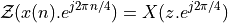
Using this transformation on the filter results in the following.

$Y(z) &= \mathcal{Z}(q[n] . e^{j 2 \pi n / 4}) \\ &= Q(z . c) \\ &= RC(z . c) . X(z^{16} . c^{16})$

In this equation, $c^{16}$ means every 16th sample from the cosine carrier, which rotates at one fourth of the sample frequency. Therefore, $c^{16} = 1$ , and the modulation output can be written as follows.

$Y(z) &= RC(z . c) . X(z^{16})$

In other words, if you take the filter coefficients of the root raised cosine filter, and you multiply them with the sequence $1, 0, -1, 0, ...$ , then you can eliminate the cosine modulator at the output! All we have to do, is to adjust the filter coefficients.

In other words, if the original raised cosine filter $RC(z)$ in C is as follows

float32_t coef[NUMCOEF] = {
                        -0.0133,
                        -0.0070,
                         0.0021,
                         0.0128,
                         0.0231,
                         0.0306,
                         0.0333,
                         0.0295,
                         0.0188,
                         0.0017,
                         ...

Then the upconverted raised cosine filter $RC(z.c)$ in C is as follows

float32_t coef[NUMCOEF] = {
                        -0.0133,
                         0.0,
                        -0.0021,
                         0.0,
                         0.0231,
                         0.0,
                        -0.0333,
                         0.0,
                         0.0188,
                         0.0,
                         ...

Optimization 2: Multirate Conversion

The second optimization is to implement an FIR filter as a multi-rate structure. The upsampled input signal has 7 zeroes for every non-zero sample. Since the overall root-raised cosine filter has 49 taps, there can be at most 7 non-zero symbols in the FIR filter at any moment in time.

Therefore, instead of building a 49-tap filter, we can just build a 7-tap filter which changes the coefficients according to the phase of the filter, where the complete filter works through 8 phases for each upsampled symbol. The following table illustrates this concept. Assume that the seven most recent symbols are stored in tap 0, 1, 2, 3, 4, 5 and 6 respectively. The filter is now going to run through 8 phases, numbered 0 to 7, to compute 8 output samples, before the next symbol will be accepted.

Phase	Tap 0	Tap 1	Tap 2	Tap 3	Tap 4	Tap 5	Tap 6
0	rrc[0]	rrc[8]	rrc[16]	rrc[24]	rrc[32]	rrc[40]	rrc[48]
1	rrc[1]	rrc[9]	rrc[17]	rrc[25]	rrc[33]	rrc[41]
2	rrc[2]	rrc[10]	rrc[18]	rrc[26]	rrc[34]	rrc[42]
3	rrc[3]	rrc[11]	rrc[19]	rrc[27]	rrc[35]	rrc[43]
4	rrc[4]	rrc[12]	rrc[20]	rrc[28]	rrc[36]	rrc[44]
5	rrc[5]	rrc[13]	rrc[21]	rrc[29]	rrc[37]	rrc[45]
6	rrc[6]	rrc[14]	rrc[22]	rrc[30]	rrc[38]	rrc[46]
7	rrc[7]	rrc[15]	rrc[23]	rrc[31]	rrc[39]	rrc[47]

In phase 0, tap 0, 1, 2, 3, 4, 5 and 6 are multiplied with filter coefficient 0, 8, 16, 24, 32, 40 and 48 respectively. This determines the first output sample.

In phase 1, tap 0, 1, 2, 3, 4, and 5 are multiplied with filter coefficient 1, 9, 17, 25, 33, and 41. Tap 6 no longer plays a role and is ignored for all subsequent phases.

This will continue for all subsequent phases. For example, the third output sample is computed as: tap0 * rrc[2] + tap1 * rrc[10] + tap2 * rrc[18] + tap3 * rrc[26] + tap4 * rrc[34] + tap5 * rrc[42].

Finally, the tap values can be updated: Tap 2 is copied to Tap 3, Tap 1 to Tap 2, Tap 0 to Tap 1 and a new symbol is read into Tap 0. Then, the sequence of sixteen phases repeats.

This multirate conversion significantly reduces the computational load of the filter, because it takes into account that most tap values of the upsampled delay line contain zeroes, and thus that we only need to care about the non-zero symbols.

Important

Question 2: Write a multirate implementation of the symbol-shaping filter that combines optimization 1 and optimization 2 explained above.

Optimization 1 can be implemented through a simple transformation of the root raised-cosine filter coefficients.

Optimization 2 will need a little more effort, in order to describe the processSample function as 16 phases that each use a different set of filter coefficients.

You will find that the major outline of the program is already set up. You only have to write an implementation of this filter in the function float32_t rrcphase(int phase, float32_t symbol). The first parameter of this function holds the current computation phase (0 to 7). The second parameter of this function holds the symbol (-1 or +1). The symbol is only valid when phase equal 0.

When your implementation is complete, capture the generated output signal on an oscilloscope. To help you record the time waveform, you can make use of the debug pin (the pin next to DAC SYNC), which is asserted by the symbol generator at the beginning of each training sequence.

In addition, capture the spectrum of the output signal. To help you capture a steady state signal, press the left button on the board. This forces the symbol generator to create an infinite stream of random symbols, which is better suited for spectrum conversion.

Step 3: Assembly Code Analysis

In the final step, you will generate assembly code for the function you just developed, rrcphase, for optimization for size. Generate an assembly listing, and look for the assembly code corresponding to rrcphase. Then, answer the following questions.

Important

Question 3: Generate assembly code for the multirate filter implementation when the compiler optimization is set of optimize for size, optimization level 2.

Include the listing for rrcphase in your report.

How many instructions do you find in the listing of rrcphase?

How many instructions execute for each invocation of rrcphase? Because of the multirate nature, the number of instructions may not be constant over all phases. In that case, count the number of instructions for phase equal to zero.

Wrapping Up

The answer to this lab consists of a written report which will be submitted on Canvas by the deadline. Refer to the General Lab Report Guidelines for details on report formatting. You will only submit your written report on Canvas. All code developed must be returned through GitHub.
Follow the principal structure of the report you’ve used for Lab 3 (taking into account any feedback you have received).
Follow the four questions outlined above to structure your report. Use figures, screenshots and code examples where appropriate. Please work out the answers in sufficient detail to show your analysis.
Make sure that you add newly developed projects to github: Use the Team - Share pop-up menu and select your repository for this lab. Further, make sure that you commit and push all changes to the github repository on GitHub classroom. Use the Team - Commit pop-up menu and push all changes.
Be aware that each of the laboratory assignments in ECE4703 will require a significant investment in time and preparation if you expect to have a working system by the assignment’s due date. This course is run in “open lab” mode where it is not expected that you will be able to complete the laboratory in the scheduled official lab time. It is in your best interest to plan ahead so that you can use the TA and instructor’s office hours most efficiently.

Good Luck

Grading Rubric

Requirement	Points
Question 1 Analysis	25
Question 2 Analysis	25
Question 3 Analysis	25
All projects build without errors or warnings	5
Code is well structured and commented	5
Git Repository is complete and up to date	5
Overall Report Quality (Format, Outline, Grammar)	10
TOTAL	100