Lab 3: Implementation of IIR filters

The purpose of this assignment is as follows.

to use the filter design tools in Matlab to create an IIR filter,
to implement the filter as a cascade structure,
to measure the filter’s performance,
to measure the filter response of the filter in two different ways:
- by measuring the impulse response in the time domain and computing the spectrum,
- by measuring the white-noise response in the time domain and computing the spectrum

Infinite Impulse Response Filter

An IIR filter is a digital filter described by the following input/output relationship

$y[n] = \sum_{k=0}^{M} b[k] x[n-k] - \sum_{k=1}^{N} a[k] y[n-k]$

where $y[n]$ is the current filter output, $b[0],...,b[M]$ are the feedforward filter coefficients, $1,a[1],...,a[N]$ are the feedback filter coefficients, and $x[n],...,x[n-M]$ are the current input and $M$ previous inputs.

An IIR filter has a feedforward order $M$ and a feedback order $N$ . In practice, $M$ and $N$ are often equal so that you can simply refer to the order of the IIR filter as meaning both feedforward and feedback order.

To compute an output of this filter, one needs to know the previous $M$ inputs as well as the previous $N$ outputs. The objective of this assignment will be to design an IIR filter and develop an implementation in C.

IIR filters they tend to require lower orders for a given filter characteristic, when compared to FIR filters. However, IIR filters have less desirable (non-linear) phase response, and their internal feedback can lead to instability. We are primarily concerned with the correct implementation of the IIR design using single-precision floating-point precision.

Infinite Impulse Response Filter Specifications

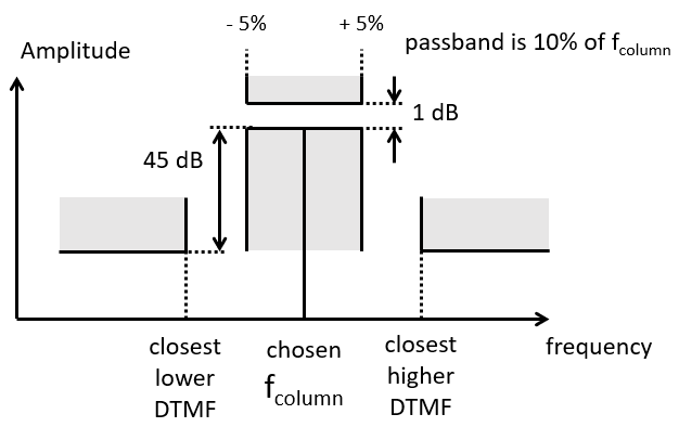
You have to design an IIR filter that can measure one of the DTMF column frequencies from other column and row frequencies. As a reminder, the DTMF column frequencies are 1209 Hz, 1336 Hz, 1477 Hz and 1633 Hz. You are free to choose what frequency you will be filtering. The passband specifications of the filter are shown in the following figure. The filter needs to provide a rejection of at least 45 dB for any DTMF frequency other than the selected column frequency. IThe passband must extend over 10% of the DTMF column frequency. For example, if you select 1477 Hz as column frequency, than the passband of your filter must be at least 147.7 Hz. The ripple in the passband frequency must be less than 1 dB.

Note

Note the following corner cases in filter specifications. If you filter 1633Hz, then the higher rejection point is fs/2. If you filter 1209 Hzm then the lower rejection point is 941 Hz.

You can use any IIR filter type you like (Butterworth, Chebyshev, Elliptic, ..) as long as it meets the specifications. It is desirable and recommended to design a filter for the lowest order possible, and for the lowest sampling frequency possible.

Important

Question 1: Using Matlab filterDesigner, create a passband filter that follows the specifications given above. For that filter, record the following properties for your report: the impulse response, the amplitude response, the phase response, and the pole-zero plot. Include each of these in your report, and clarify the design constraints you have used for your design. In addition, export the filter coefficients in single-precision floating point accuracy. An IIR filter is typically implemented as a cascade structure of second-order coefficients.

Infinite Impulse Response Filter Implementation

The second part of the lab is to implement the filter using a C program. You will implement the filter as a transpose direct-form II structure using second-order-stages (SOS).

The format of the include files generated by Matlab deserves a closer look. Here is an example of a fourth-order Butterworth filter generated as two second-order-stages (SOS).

#define MWSPT_NSEC 5
const int NL[MWSPT_NSEC] = { 1,3,1,3,1 };
const real32_T NUM[MWSPT_NSEC][3] = {
  {
     0.4433953762,              0,              0
  },
  {
                1,              0,             -1
  },
  {
     0.4433953762,              0,              0
  },
  {
                1,              0,             -1
  },
  {
                1,              0,              0
  }
};
const int DL[MWSPT_NSEC] = { 1,3,1,3,1 };
const real32_T DEN[MWSPT_NSEC][3] = {
  {
                1,              0,              0
  },
  {
                1,   -1.159571767,   0.5372180343
  },
  {
                1,              0,              0
  },
  {
                1,   0.2169253677,   0.3766086996
  },
  {
                1,              0,              0
  }
};

This filter is created using five second-order sections (MWSPT_NSEC).
The NUM array contains the numerator of the transfer function, and it holds the b[k] coefficients. The DEN array contains the denominator of the transfer function, and it holds the a[k] coefficients.
There are five rows in each of NUM and DEN. Each second-order stage uses two rows, while the final row describes a global gain $G$ . The transfer function of the filter can be described as $H[z] = \frac{GN . ( N1[z] . N2[z] )}{GD . ( D1[z] . D2[z] )}$ . where $\frac{N1[z]}{D1[z]}$ is the first second-order stage, $\frac{N2[z]}{D2[z]}$ is the second second-order stage, and $\frac{GN}{GD}$ is the global gain $G$ .
In each row pair that captures a second-order stage, the first row represents a gain while the second row represents the filter coefficients. For example, the first two rows of NUM specify the following transfer function: $N1[z] = 0.4433953762 . ( 1 + 0.z^{-1} - 1.z^{-2} )$ .

  const real32_T NUM[MWSPT_NSEC][3] = {
  {
     0.4433953762 /* N0 */,              0,              0
  },
  {
                1 /* b0 */,              0 /* b1 */,             -1 /* b2 */
  },

Similarly, the first two rows of DEN specific the following transfer function: $D0[z] = 1 . ( 1 - 1.159571767.z^{-1} + 0.5372180343.z^{-2} )$ .

  {
                1 /* D0 */,              0,              0
  },
  {
                1 /* a0 */,   -1.159571767 /* a1 */,   0.5372180343 /* a2 */
  },

The last row of both NUM and DEN specify an overall gain factor

Important

Question 2: Next, write a C program implementation of a transpose direct-form II bandpass filter according to the specifications of DTMF bandpass filter designed in Question 1. Demonstrate that your filter can operate in real time as follows. First, use the xlaudio_measurePerfBuffer() function to determine the cycle count of your filter execution time. Refer to the FIR examples on GitHub to see how to use this function. Second, measure the period of the DAC_SYNC signal on pin J2.12 of the pin header on the BOOSTXL_AUDIO board. Show that the period matches the sample frequency chosen for your application.

Note

It’s a good idea to try to use the coefficients directly as generated from the Matlab include file. The include file generate from Matlab’s filter designer defines a single-precision floating point type as real32_T whereas the ARM DSP library uses the float32_t. It also makes use of an external include file twmtypes.h. You can either cut-and-paste the coefficient values into your C program, or else include the generated coefficient file and ensure that the C compiler understands that real32_T and float32_t are the same data type.

Infinite Impulse Response Filter Evaluation

In the second half of the lab, you will evaluate the frequency response of the filter. You will do this in two different ways. The first is to measure the impulse response in the time domain, and compute the spectrum of the resulting wave form. The second is the measure the response to a noise signal in the time domain, and compute the spectrum of the resulting waveform. You will record both of these spectra and compare them to the theoretical (noiseless) spectrum obtained from Matlab’s filterDesigner.

Spectrum Response from an impulse

In the time domain, we can mimic a single impulse through a pulse wave with a very low duty cycle, say 1 %. The period of the pulse wave stimulus has to be large enough for the IIR filter (which is, theoretically, infinite in length) to die out below the quantization threshold of the DAC.

In the lab code, the function impulseresponse shows how this pulse wave can be created.

uint16_t impulseresponse(uint16_t x) {
  float32_t input;
  static int k = 0;
  k = k + 1;
  if (k == 500) {
      k = 0;
      xlaudio_debugpinhigh();
      input = 0.2;
  } else {
      xlaudio_debugpinlow();
      input = 0;
  }

  return xlaudio_f32_to_dac14(transposefilter(input));
}

This function is called through a periodic interrupt at the sample rate. Every 500 calls, the function assigns the value 0.2 to input. In all other instances, the value 0 is assigned. Hence, we are creating a pulse wave with a duty cycle of 1/500 and a period of (sample rate / 500). It depends on your design to fine tune the parameter 500 (and the pulse height 0.2) to fit your application. If all goes well, you will be able to capture the impulse response of the filter on the DAC output.

In addition, a digital version of the pulse is also created on the debug pin. This is a dedicated pin on the BOOSTXL-AUDIO board, mapped to GPIO 3.5 (port 3 bit 5). On the BOOSTXL-AUDIO board, this pin maps to header J4 pin 30. The idea of this pin is to serve as a trigger for the oscilloscope that will measure the impulse response.

To compute the spectrum of the resulting impulse response, you can either directly use the spectrum analyzer function of the Analog Discovery scope, or else capture the waveform itself from a storage scope, and compute the spectrum in Matlab.

Important

Question 3: Measure the spectrum of the impulse response of your IIR filter through the pulse generation method. Compare the result with the ‘ideal’ spectrum computed by Matlab. Analyze and comment on any differences you find. For this lab, we are only focusing on the amplitude response; you can ignore the phase response.

Spectrum Response from noise stimulus

A second method to measure the amplitude response of a filter is to mimic an impulse as a white-noise (random) signal. Such a signal is equivalent to a dirac impulse, but has random phase rather than zero-phase and hence appears as a random waveform in the time domain instead of as an impulse.

In the lab code, the function noiseresponse show how this waveform can be created.

uint16_t noiseresponse(uint16_t x) {
    x = rand() % 1024; // 10-bit noise
    float32_t input = xlaudio_adc14_to_f32(0x2000 - (0x1000 / 2) + x);

    return xlaudio_f32_to_dac14(transposefilter(input));
}

The function is called through a period interrupt at the sample rate. The value of the signal is defined as a random 10-bit number, with an offset to account for the DAC14 calibration on the AUDIO-BOOSTXL board. When applying this noisy signal to the input, you will observe a filtered version at the DAC output. Since the input spectrum is white (uniform), the spectrum of the output signal is equivalent to the amplitude response of the filter.

To compute the spectrum of the resulting impulse response, you can proceed in the same fashion as you did with the impulse response. You can either directly use the spectrum analyzer function of the Analog Discovery, or else capture the waveform itself from a storage scope, and compute the spectrum in Matlab.

Important

Question 4: Measure the spectrum of the impulse response of your IIR filter through the noise generation method. Compare the result with the ‘ideal’ spectrum computed by Matlab. Analyze and comment on any differences you find. For this lab, we are only focusing on the amplitude response; you can ignore the phase response.

In addition, also compare the three spectra relative to each other: the theoretical spectrum from Matlab, the measured spectrum from the impulse response, and the measured spectrum from the noise response. Analyze and command on any differences you finds.

Attention

Measuring a spectrum accurately is a difficult task, harder than measuring for example the time domain response. Take your time for each of Question 3 and Question 4 to understand and analyze what you see. You may not be able to reproduce the theoretical spectrum of Matlab exactly, and that’s okay. They key objective is to build insight into the factors that contribute to the differences.

Wrapping Up

The answer to this lab consists of a written report which will be submitted on Canvas by the deadline. Refer to the General Lab Report Guidelines for details on report formatting. You will only submit your written report on Canvas. All code developed must be returned through github.
Follow the principal structure of the report you’ve used for Lab 3 (taking into account any feedback you have received).
Follow the four questions outlined above to structure your report. Use figures, screenshots and code examples where appropriate. Please work out the answers in sufficient detail to show your analysis.
Make sure that you add newly developed projects to github: Use the Team - Share pop-up menu and select your repository for this lab. Further, make sure that you commit and push all changes to the github repository on GitHub classroom. Use the Team - Commit pop-up menu and push all changes.
Be aware that each of the laboratory assignments in ECE4703 will require a significant investment in time and preparation if you expect to have a working system by the assignment’s due date. This course is run in “open lab” mode where it is not expected that you will be able to complete the laboratory in the scheduled official lab time. It is in your best interest to plan ahead so that you can use the TA and instructor’s office hours most efficiently.

Good Luck

Grading Rubric

Requirement	Points
Question 1 Analysis	15
Question 2 Analysis	10
Question 3 Analysis	20
Question 4 Analysis	25
All projects build without errors or warnings	5
Code is well structured and commented	5
Git Repository is complete and up to date	5
Overall Report Quality (Format, Outline, Grammar)	15
TOTAL	100