Digital Modulation ¶

Contents

Digital Modulation

The purpose of this lecture is as follows.

To describe DSP implementation aspects of digital modulation
To explain the design and implementation of multi-rate digital filters

Digital Modulation ¶

One of the very important application domains for Digital Signal Processing is the domain of Data Transmission. Examples include wireless communications, Ethernet, digital telephony, optical fiber communications, etc. Our department has a separate course on Principles of Communication Systems (ECE 3311), which also covers data transmission.

In this lecture, we will study some of the DSP implementation aspects of data transmission. This material will be useful, in part, to address the final labs in the course. Since we are spending just one (or two) lectures on data communications, the treatment of the subject is very brief and very incomplete. Think of this material as an illustration that shows how DSP is used in practice.

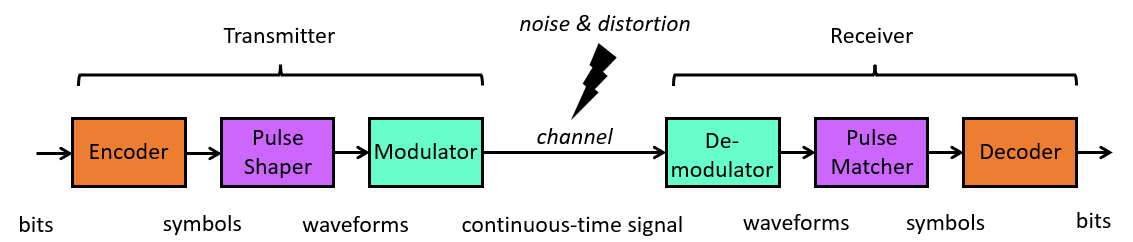
This figure shows a highly simplified view of a data communications system. The overall objective is to transmit bits from the transmitter to the receiver over a channel. The channel is subject to noise and distortion, and moreover the channel is only capable of carrying analog (continuous-time) quantities such as a voltage waveform, or an electromagnetic wave.

The transmitter therefore goes through a three-step process to convert discrete bits into an analog waveform.

First, bits are encoded into symbols. A symbol is the unit of information that is transmitted over the channel. Each symbol contains a predefined number of bits. The input to the encoder is a stream of bits at a given bitrate (bits/second). The output of the encoder is a stream of symbols at a given symbolrate (symbols/second). When each symbol encodes a single bit, obviously, the symbolrate and the bitrate are identical.
Next, each symbol (which is still a discrete quantity) is converted to a smooth waveform by the pulse shaper. If the pulse shaper is an analog circuit, the output of the pulse shaper is a continuous-time signal. If the pulse shaper is a digital circuit (such as a digital filter), the output of the pulse shaper is a discrete-time signal. However, the sample rate at the pulse shaper output will be typically much higher than the symbol rate. The smooth waveform at the output of the pulse shaper is also called a baseband signal, as it contains frequencies between DC and (a little bit more than) the symbol rate.
Third, the baseband signal is modulated to make it suitable for transport over the channel. Modulation combines the baseband signal with a carrier signal, such that the baseband signal is used to control the amplitude, or phase, or frequency of the carrier signal. This results in amplitude, resp. phase, resp. frequency modulation. In analog transmitters, the modulation circuit is analog. However, the modulation process can be implemented as a digital signal processing (DSP) operation as well. For example, in software radios, the modulation step is performed by digital hardware or DSP processors.

At the receiver, the modulated signal is converted back into bits through the opposite sequence of steps.

First, the carrier signal is removed in the demodulator. Some demodulation schemes require knowledge of the exact frequency and phase of the carrier used by the transmitter. These schemes are called coherent modulation schemes. When the exact frequency or phase is not needed, the modulation scheme is non-coherent. In coherent receivers, the carrier frequency and phase are often reconstructed using (DSP) operations on the received signal, in a process called carrier synchronization.
Second, the resulting demodulated waveform is processed by a pulse matcher or matching filter. The objective of the receiver is to look for the pulse shapes used by the transmitter to represent symbols. This involves finding the starting point of a pulse shape, a process known as symbol timing synchronization.
Finally, the bits are decoded from the received symbol in order to reconstruct the bit stream sequence used at the transmitter. Advanced encoding schemes may also include error correction, which accounts for the degradation of the transmitted signal by channel distortion and noise.

There are many different techniques for modulation and pulse shaping, and we will only discuss a very select few of them. However, regardless of the modulation scheme used, every (digital) communication system has similar overall objectives.

First, one wishes to minimize the number of bit errors. The residual number of bit errors is expressed in the bit error rate, the number of bit errors occuring per N transmitted bits.
Second, one wishes to maximize the efficiency of the transmission by cramming as many bits as possible per unit of bandwidth. Communication systems are therefore also characterized by their spectral efficiency, which is the number of bits/second that can be transmitted per Hertz of bandwidth in the communication channel.

Digital Modulation Mechanisms with an Analog Carrier ¶

In this lecture, we only consider modulation schemes for digital data over an analog carrier. The analog carrier is characterized by a cosine with a specific amplitude, frequency and phase.

$c(t) = A_c cos(2 \pi f_c t + \theta_c)$

The amplitude, frequency and phase are three parameters on the carrier that can be varied under influence of a symbol shape.

In an amplitude modulation scheme, the carrier amplitude $A_c$ is changed as a function of the symbol pulse shape.
In a frequency modulation scheme, the carrier frequency $f_c$ is changed as a function of the symbol pulse shape.
In a phase modulation scheme, the carrier phase $\theta_c$ is changed as a function of the symbol pulse shape.

Three common modulation schemes are Amplitude Shift Keying (ASK), Phase Shift Keying (PSK) and Frequency Shift Keying (FSK). These schemes directly map a binary symbol (0 or 1) into a carrier waveform, using only a very trivial pulse shaping step such as a rectangular pulse. The following table expresses the carrier waveform for each case when transmitting a ‘0’ bit ( $s_1(t)$ ) and ‘1’ bit ( $s_2(t)$ ) respectively.

Scheme	$s_1(t)$	$s_2(t)$
ASK	0	$A cos(\omega t)$
PSK	$A cos(\omega t + \beta)$	$A cos(\omega t - \beta)$
FSK	$A cos(\omega t )$	$A cos((\omega + \delta) t)$

The binary ASK and binary FSK schemes, in particular, are popular in low-cost (high-volume) applications such as garage door openers.

We will study Binary Phase Shift Keying in further detail.

Binary Phase Shift Keying (BPSK)¶

A BPSK signal uses two symbols with values +1 and -1 respectively. The pulse shape of a BPSK signal is, in its simplest form, a rectangular pulse of $T$ seconds wide.

The baseband signal that is generated for the modulator is therefore a signal of the following form.

$d(t) = \sum_k b_k p(t - kT)$

where $b_k$ is a symbol sequence containing the symbols +1 and -1, and $p(t)$ is a rectangular pulse of unit height.

In BPSK modulation, the baseband signal $d(t)$ is used to vary the phase of a carrier signal between 0 and 180 degrees. Thus, the modulated signal has the following form.

$s(t) = d(t) cos(2 \pi f_c t)$

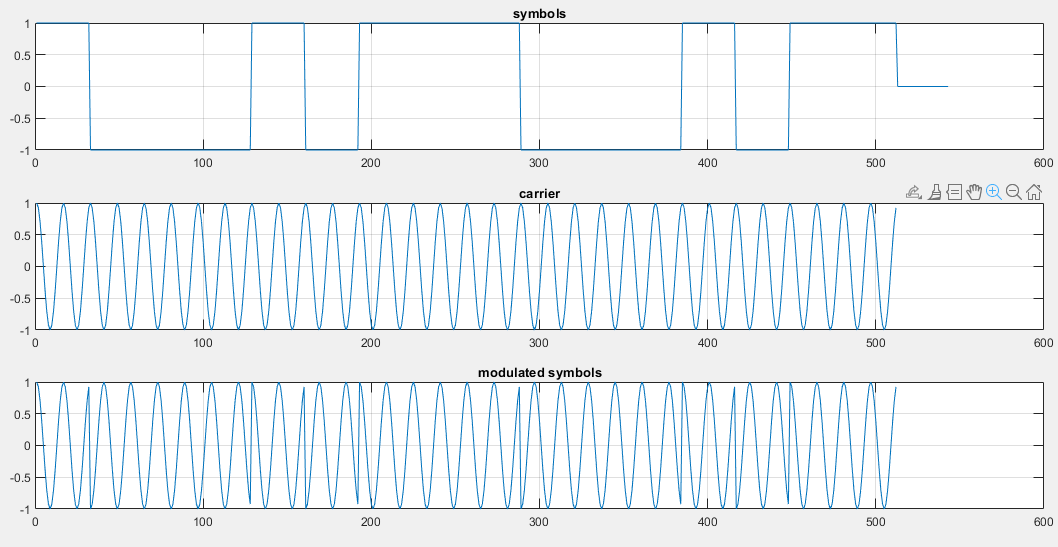
The following figure illustrates an example of a symbol waveform $d(t)$ , and a modulated symbol waveform $s(t)$ . The phase transitions from symbol to symbol are quite abrupt, and this will contribute the extra bandwidth (and reduced spectral efficiency).

To study the spectrum of the modulated BPSK signal, we can use Matlab. We set up a discrete time simulation as follows. We use 16 samples per symbol, and a carrier frequency of one fourth of the sample frequency. Then, we generate 160 random symbols and compute the spectrum of the baseband signal and the modulated signal using pwelch. The following code achieves this objective.

samplespersymbol = 16;      % simulation done at this number of samples per symbol
numsymbols       = 160;      % simulate this number of symbol
carrierfreq      = 4;       % times the symbol frequency; <= samplespersymbol

carriersync      = [ 1 -1 -1 -1  1 -1  1 1];

sync1    = [carriersync carriersync ];
payload  = (floor((rand(numsymbols-length(sync1),1) * 2)) - 0.5) * 2;
symbols  = [sync1'  ; payload];

carrier          = cos(2 * pi * carrierfreq*((1:samplespersymbol)-1)/samplespersymbol);

fullcarrier      = repmat(carrier', numsymbols, 1);     % '
symsignal        = repelem(symbols, samplespersymbol);
upsym            = conv(upsample(symbols, samplespersymbol), ones(samplespersymbol,1));

% convolution of a[n] and b[m] gives a signal of length m + n - 1
% however, the last m-1 values of a[n] are zero (as a[n] is the upsampled symbol stream)
% we therefore cut off conv(a,b) at length n
modsym           = fullcarrier .* upsym(1:(samplespersymbol*numsymbols));

figure(1)
pwelch(upsym(1:(samplespersymbol*numsymbols)))
figure(2)
pwelch(modsym)

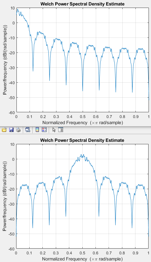
From the spectrum, we see that the main lobe of the baseband signal has with $f_s/16$ (the fractional bandwidth is 0.125, with half the sample frequency located at 1), and that it has a sincx rolloff. This means that the baseband signal has a relatively high bandwidth. The modulated signal is centered around the carrier frequency $f_s/4$ . The main lobe has width $f_s/8$ , as BPSK uses a double-sideband format.

Pulse Shaping for BPSK ¶

In a BPSK scheme with symbols shaped as rectangular pulses, there are severe discontinuities in the modulated waveform. These discontinuities are a direct consequence of the +1/-1 amplitude jumps in the baseband signal. The net effect is that the bandwidth of the modulated signal is significantly wider than the symbol rate.

We can do reduce that extra bandwidth by applying pulse shaping to the baseband signal. Instead of using a rectangular waveform, we will use a waveform which smoothly interpolates in between the sequence of symbol values. The ideal interpolator for a stream of pulses is a $sin(x)/x$ shape. The following figure illustrates such sincx interpolation.

We are transmitting the symbol sequence +1, -1, +1, +1. The blue curve shows the baseband signal with rectangular pulse shaping. Instead, we replace each rectangular pulse with a sincx shape. The width of the sincx is chosen such that the zeros of one pulse shape coincide with all symbol locations except one - the symbol on which the sincx is centered. The interpolated waveform, shown in red, is the sum of all these sincx shapes superimposed over one another. Clearly, this interpolated waveform has to hit every symbol at +1 or -1, while at the same time providing a smooth transition from one symbol to the next.

It can be shown that the red curve has the lowest bandwidth of every possible interpolated curve. Recall that the spectrum of a rectangular shape (in the frequency domain) corresponds to a $sin(x)/x$ shape in the time domain. In the frequency domain, the sincx corresponds to an ideal lowpass filter with cutoff frequency equal to the symbol rate.

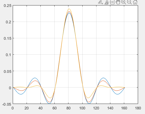
The main disadvantage of such a sincx interpolation filter is that it has a slow dropoff in time, and therefore requires a very long interpolation filter. It also increases latency, since each pulse shape now extends over multiple symbol periods. BPSK systems therefore make use of a pulse shaping filter that has a faster dropoff in the time domain. In the frequency domain, this new filter has a raised-cosine transition band rather than a steep brickwall transition band. It is aptly named a raised cosine filter. The raised-cosine thus refers to the transition band in the frequency domain. The raised-cosine filter introduces one extra parameter r, the rolloff factor, which characterizes the extra bandwidth of the filter beyond the brick-wall bandwidth. A rolloff factor of 1 means that the raised-cosine filter has twice the symbol bandwidth; a rolloff factor of 0.25 means that the raised-cosine filter has 1.25 times the symbol bandwidth. The following figure shows the time-domain raised-cosine impulse response at roll-off factors 0 (blue), 0.25 (red) and 0.5 (yellow).

Digital Pulse Shaping Filter ¶

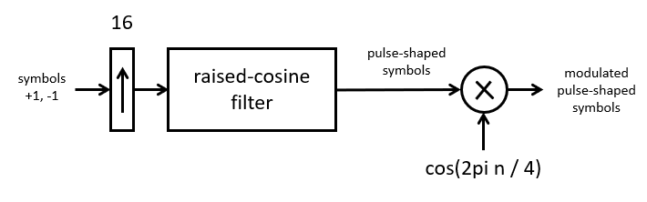
We now develop a fully digital version of a BPSK modulator with a raised-cosine pulse shaper. The pulse shaping filter of the BSPK modulator is a multi-rate filter. Such a filter has a different sample rate at its input compared to its output. In the case of the BPSK pulse shaping filter, the input sample rate is determined by the symbol rate, while the output sample rate is determined by the number of samples per symbol used for the modulation scheme.

In the following, we aim to develop both the pulse shaper as well as the modulator as a DSP function. Therefore, we select a sample rate which is fast enough to represent both the baseband waveform as well as the modulated waveform. We select a sample rate of 16 times the symbol frequency. We use a carrier frequency of 4 times the symbol frequency. The carrier frequency is thus one fourth of the sample frequency. These parameter selections correspond to the parameter selections used by Lab 5.

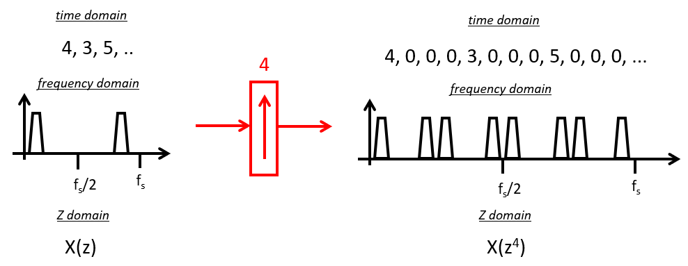
To describe multirate digital filters, we need a new DSP primitive: the upsampler. An upsampler is a module that injects zeroes in between the samples of an input stream. An N-fold upsampler injects N-1 zeroes for every input sample. The following shows the example of a 4-fold upsampler. In an input stream of sample values 4, 3, 5, it will inject three zeroes in between every sample value to produce the output stream 4, 0, 0, 0, 3, 0, 0, 0, 5, 0, 0, 0. The upsampler also has a well defined effect in the frequency domain as well as in the Z-transform domain.

At 16 samples per symbol, we need a 16-fold upsampler, so the following figures will show a 16-fold upsample operation instead. The upsampler is used in combination with an interpolation filter (pulse shaper), and a double side band modulator, to create the modulated waveform. Note that the discrete-time version of a modulator is now given by a discrete-time cosine $cos(2 \pi n /4)$ , where $n$ is the sample index. This particular modulator will produce the values 1, 0, -1, 0, 1, .. and so forth, which makes the multiplication operation trivial.

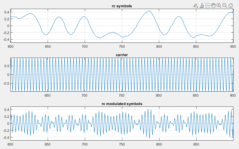
To study the spectrum of the modulated pulse-shaped BPSK signal, we again use Matlab. The following code achieves this objective. The spectrum of the pulse-shaped BSPK signal now is limited to a central band width approximately equal to the symbol rate. This interpolation filter is 5 symbols long at 16 samples per symbol, resulting in a FIR with 80 (+1) taps. In lab 5, a 3-symbol interpolation filter is used, which results in a FIR of 48 (+1) taps.

samplespersymbol = 16;      % simulation done at this number of samples per symbol
numsymbols       = 160;      % simulate this number of symbol
carrierfreq      = 4;       % times the symbol frequency; <= samplespersymbol

carriersync      = [ 1 -1 -1 -1  1 -1  1 1];

sync1    = [carriersync carriersync ];
payload  = (floor((rand(numsymbols-length(sync1),1) * 2)) - 0.5) * 2;
symbols  = [sync1'  ; payload];

carrier          = cos(2 * pi * carrierfreq*((1:samplespersymbol)-1)/samplespersymbol);

fullcarrier      = repmat(carrier', numsymbols, 1);     % '

rcpulse          = rcosdesign(0.25, 5, samplespersymbol, 'normal');
rcupsym          = conv(upsample(symbols, samplespersymbol), rcpulse);
modrcsym         = fullcarrier .* rcupsym(1:(samplespersymbol*numsymbols));

figure(1)
pwelch(rcupsym(1:(samplespersymbol*numsymbols)))
figure(2)
pwelch(modrcsym)

Efficient Implementation of the Digital BPSK Modulator ¶

We can finally implement the digital BPSK modulator. In the implementation, we try to minimize the amount of effort (data computations, data movement) spent in the software. For example, for a multiplication with a sequence 1, 0, -1, 0, 1, .. it doesn’t pay off to use a full multiplier. Instead, we can simply clear half the output samples, and flip the sign of half of the remaining non-zero ones.

Efficient Implementation of the Modulation Operation ¶

However, we can do even better than that. We make use of the following property (scaling of the Z transform):

$\mathcal{Z}(x(n) . e^{j 2 \pi n / 4}) = X(z . e^{j 2 \pi / 4})$

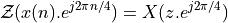
That is, if we know $X(z) = x_0 + x_1 . z^{-1} + x_2 . z^{-2} + x_3 . z^{-3} + ..$ , then $X(z . e^{j 2 \pi / 4}) = x_0 + j.x_1.z^{-1} - x_2.z^{-2} - j.x_3.z^{-3} + ..$ .

For a cosine at $fs/4$ , the coefficients in $X(z)$ are multiplied with the sequence $1, 0, -1, 0, 1, 0, ....$ . We will use the notation $X(z . c)$ to indicate this transformation.

Using this transformation on the filter results in the following.

$Y(z) &= \mathcal{Z}(q[n] . e^{j 2 \pi n / 4}) \\ &= Q(z . c) \\ &= RRC(z . c) . X(z^{16} . c^{16})$

In this equation, $c^{16}$ means every 16th sample from the cosine carrier, which rotates at one fourth of the sample frequency. Therefore, $c^{16} = 1$ , and the modulation output can be written as follows.

$Y(z) &= RRC(z . c) . X(z^{16})$

In other words, if you take the filter coefficients of the root raised cosine filter, and you multiply them with the sequence $1, 0, -1, 0, ...$ , then you can eliminate the cosine modulator at the output! All we have to do, is to adjust the filter coefficients.

Efficient Implementation of the Multirate Filtering ¶

Another opportunity for optimization is the implementation of the multirate filter. For every non-zero sample, the upsampler operation feeds on 15 zeros into the pulse shaping filter. Hence, most of the coefficient multiplications performed in this filter can be skipped. The following figure illustrates how a filter with an upsampler of 4 can be optimized.

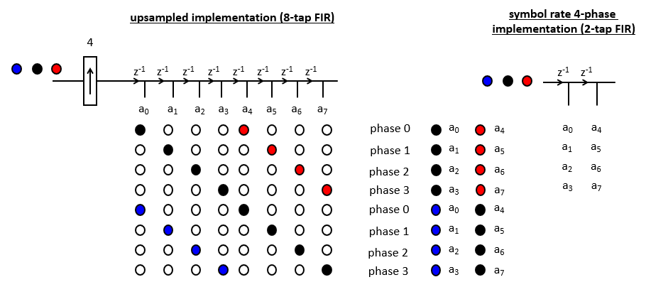
In the traditional implementation (left), there are only two non-zero samples in an 8-tap filter. Hence, the effective work that has to be performed by the filter is only two coefficient multiplications per input sample at the high rate.

Therefore, we reformulate the filter’s operation as moving through 4 phases, each representing one phase of the upsample operation. This allows a reformulation of the delay line at the low rate (right), where each new sample is subject to 4 phases. This multirate filter is now performing only the multiplications that are strictly needed, and avoiding useless multiplications with zero, as well as useless storage of zero-samples.

Formulating a filter as a multirate implementation requires the C code to take into account the phase of the filter. The following is an example of an non-optimized filter that accepts an upsampled signal.

static int phase = 0;

// traditional implementation
float32_t taps[NUMCOEF];
uint16_t processSample(uint16_t x) {
    float32_t input = xlaudio_adc14_to_f32(x);

    // the input is 'upsampled' to RATE, by inserting N-1 zeroes every N samples
    phase = (phase + 1) % RATE;
    if (phase == 0)
        taps[0] = input;
    else
        taps[0] = 0.0;

    float32_t q = 0.0;
    uint16_t i;
    for (i = 0; i<NUMCOEF; i++)
        q += taps[i] * coef[i];

    for (i = NUMCOEF-1; i>0; i--)
        taps[i] = taps[i-1];

    return xlaudio_f32_to_dac14(0.1 * q);
}

The phase is captured in the phase variable, which will let the input to be nonzero only one out of RATE samples. However, the filter computation itself is not multirate, as it will perform NUMCOEF multiplications of all coefficients and all taps, regardless of wether the taps contain the value zero or not.

Therefore, we improve the code with a shorter delay line of only NUMCOEF/RATE + 1 taps, and using the phase variable to control which coefficients are used to compute the output. The following code shows the multirate version of the single rate filter listed above.

float32_t symboltaps[NUMCOEF/RATE + 1];

uint16_t processSampleMultirate(uint16_t x) {
    float32_t input = xlaudio_adc14_to_f32(x);

    phase = (phase + 1) % RATE;

    uint16_t i;
    if (phase == 0) {
        symboltaps[0] = input;
        for (i=NUMCOEF/RATE; i>0; i--)
            symboltaps[i] = symboltaps[i-1];
    }

    float32_t q = 0.0;
    uint16_t limit = (phase == 0) ? NUMCOEF/RATE + 1 : NUMCOEF/RATE;
    for (i=0; i<limit; i++)
        q += symboltaps[i] * coef[i * RATE + phase + 1];

    return xlaudio_f32_to_dac14(0.1 * q);
}

The example code of this lecture compares both implementations from a performance point of view. With the optimization-for-size flag set at level two, the single-rate filter consumes 920 cycles per sample, while the multi-rate filter consumes only 345 cycles per sample. That’s an improvement of 2.66 times. With higher upsample rates (such as the upsample factor of 16 as used in Lab 5), the improvements will be even better.

Conclusions ¶

The key objective of this lecture was to explain how DSP techniques can be used in the implementation of digital communication systems. In this lecture, we discussed the design of BPSK modulation with pulse shaping. We then discussed two important DSP optimization techniques for implementation: multirate expansion, and coefficient rotation optimization. In the following lecture, we will discuss a technique to demodulate these BPSK signals.