Linear Phase in Communication ¶

Contents

Linear Phase in Communication

The purpose of this lecture is as follows.

To explain the difference between IIR and FIR filters from the perspective of phase
To illustrate that difference using an example of a communication system
To demonstrate the impact of linear phase empirically in a Matlab simulation

FIR or IIR ¶

In the past two lectures, we discussed standard implementation techniques for FIR and IIR filters: direct-form, and their transposed implementations, and then two decomposed forms including cascade and parallel design. If you’ve experimented with such filters in Matlab, you will have noticed that in general, IIR filters are much lower order than FIR filters under the same amount of filtering. ‘Filtering’, in this context, means the ability to suppress a given frequency by x dB, or the ability to implement a transition band between bandpass and bandstop at a given steepness.

IIR filters achieve lower order by strategically placing poles, which allow the frequency response of a transfer function $G(z)$ to be boosted by a significant amount. In contrast, FIR filters can only weaken the frequency response by adding more zeroes.

From a computational and implementation-efficiency perspective, we would therefore be tempted to conclude that IIR filters are preferable over FIR filters. IIR filters will requires less software instructions, or less hardware gates, for the same amount of filtering as an equivalent FIR filter.

However, there is an important difference between FIR and IIR filters. FIR can have a linear phase response. That means that the phase is a linear function of the frequency. This property occurs when the FIR filters have a symmetric impulse response. In contrast, IIR filters have a non-linear phase response. The phase response of an IIR may contain non-linear terms in their frequency response, such as quadratic, cubic, and higher-order terms. In the following example, we investigate the impact of non-linear phase in an application domain where the phase response plays an important role, namely in the design of communication systems.

Double-side band modulation ¶

In a modulation system, a source signal $x(t)$ is converted from baseband to passband. Baseband contains the frequencies between DC and the highest frequencies in $x(t)$ . Passband contains a range of frequencies around a carrier frequency $f_c$ . The modulation process shifts the baseband spectrum of $x(t)$ to the carrier frequency $f_c$ , such that the old ‘DC’ frequency maps to the carrier frequency $f_c$ . Once the signal is in passband, it can be transmitted over a channel. Modulation is commonly used in radio. For example, $x(t)$ is a music signal, and the carrier frequency $f_c$ is the radio frequency that you’d use on the radio to tune into that station.

At the receiver side, the passband signal is converted back to baseband. This involves shifting the spectrum of the modulated signal down to DC, in order to restore a baseband signal $y(t)$ . Ideally, the resulting signal $y(t)$ is identical to the original input signal $x(t)$ , with minimal distortion. Often, transmission over a channel will inject noise. In this case, however, we will assume there is no noise.

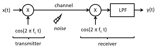
We will study a specific modulation system called double-side band modulation. Its structure is shown in the following figure. $x(t)$ is first multiplied with a cosine of frequency $f_c$ . The resulting passband signal is then transported to the receiver over the channel. At the receiver, the signal is again multiplied with the carrier frequency. Finally, a lowpass filter is used to create the reconstructed basedband signal $y(t)$ . Two remarks on this design: (1) The signal processing chain is in continuous-time; we will present a discrete-time version later. (2) The carrier at the receiver has exactly the same frequency and phase as the carrier at the transmitter. This is an idealized situation, and in a real radio there is special circuitry to reconstruct the receiver carrier as an identical (frequency, phase) copy of the transmitter carrier. In this example, we assume that this problem is already solved.

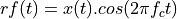
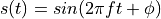
The following steps show mathematically how the modulation and demodulation process works. First, the RF signal is created by multiplying $x(t)$ with $cos(2 \pi f_c t)$ .

$rf(t) = x(t) . cos(2 \pi f_c t)$

Next, the signal is downconverted again to baseband.

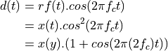
$d(t) &= rf(t) . cos(2 \pi f_c t) \\ &= x(t) . cos^2(2 \pi f_c t) \\ &= x(y) . (1 + cos(2 \pi (2 f_c) t))$

To derive $d(t)$ , we relied on the identity 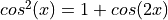$cos^2(x) = 1 + cos(2x)$ . The downconverted signal thus contains two copies of $x(t)$ : one at the baseband frequency, and a second one which is modulated at twice the carrier frequency $f_c$ . This explains the role of the lowpass filter following the downconversion. The lowpass filter will remove the second copy of $x(t)$ located at a high passband frequency. Thus, ideally, with a good lowpass filter, the image $y(t)$ is almost identical to x(t).

$y(t) &= LPF(d(t)) \\ &= LPF(x(t) (1 + cos(2 \pi (2 f_c) t))) \\ &= LPF(x(t))$

Double-side band modulation of a square wave ¶

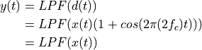
In the following, we will assume an example $x(t)$ in the form of an approximated square wave. A square wave, symmetrical around the x-axis, can be approximated as a sum of sines. Namely:

$square(t) = sin(2 \pi f t) + \frac{sin(2 \pi (3.f) t)}{3} + \frac{sin(2 \pi (3.f) t)}{5} + ..$

As more terms that are included in this series, the square wave shape will be approximated in more detail. The following figure shows the shape of the square wave when the first three harmonics are added together. While the resulting waveform is far from a square wave shape, it’s clear that the sum of three harmonics is a better approximation of a square wave than, say, the base harmonic by itself. This signal $x(t)$ has a spectrum that consists of three dirac impulses, located at f, 3f, and 5f, and with area 1, 1/3 and 1/5 respectively. In addition, all harmonics are precisely in phase. The sharp rising edge of the square wave is possible because all harmonics together go through phase = 0 and start increasing from there.

In the following, we will choose concrete frequencies for the carrier frequency and the square wave frequency, and we will model the double-side band modulation process as a discrete-time signal processing problem. We choose a sample frequency of 60KHz and a base square wave frequency of 1 KHz (1/60th of the carrier). This puts the harmonics at 3 KHz and 5 KHz, respectively. We also select a carrier frequency of one fourth of the sample frequency, or 15 KHz.

The following matlab code shows how to up-convert the baseband signal, and downconvert it again.

x = [1:1024];

clf;
hold off;

% create pulse waveform
base = 1;     // ground frequency multiplier
sq = sin(base * 2 * pi / 60 * x) + sin(base * 2 * pi / 20 * x) / 3 + sin(base * 2 * pi / 12 * x) / 5;
figure(1)
plot(sq)

% create the modulated signal
carrier = cos(2 * pi / 4 * x);
rf      = carrier .* sq;
figure(2)
subplot(3,1,1)
plot(abs(fft(sq)))
title('Baseband Amplitude Spectrum')
subplot(3,1,2)
plot(abs(fft(rf)))
title('RF Amplitude Spectrum')

% downconvert the modulated signal
dc    = rf .* carrier;
figure(2)
subplot(3,1,3)
plot(abs(fft(dc)))
title('Downconverted signal spectrum')

The spectrum of the baseband signal, the passband signal, and the downconverted passband signal, clearly show the three peaks that make up the (partial) square wave. The spectrum is computed using the Fast Fourier Transform, and show the baseband and a negative image at the sample frequency (which corresponds to what we expect for discrete-time systems.) The modulation at a carrier frequency of one fourth of the sample frequency creates two bandpass signals, one around $fs/4$ and a corresponding image around $3 fs/4$ . The double-sideband nature of the modulated signal is visible, as the original baseband signal, stretching from DC to 5KHz, is transformed into a bandpass signal stretching from 10 KHz to 20 KHz. There is an additional image band from 40 KHz to 50 KHz. Aftter the downconversion step, the original baseband signal is restored, but there are additional components located around twice the carrier frequency $2.f_c = 2.f_s = 30 KHz$ . 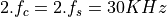To reconstruct the original input signal $x(t)$ , a low-pass filter is needed.

DSB demodulation Lowpass filter design ¶

In order to recover the original signal from the demodulated signal, we will use a lowpass filter with a cutoff frequency of $fs/4$ . We would also like this filter to be steep. A steep transition band will allow the baseband signal bandwidth to be as broad as possible, while still suppressing the image band centered around $fs/4$ . Hence, we settle for the following specs.

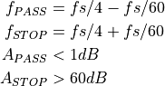
$f_{PASS} &= fs/4 - fs/60 \\ f_{STOP} &= fs/4 + fs/60 \\ A_{PASS} &< 1 dB \\ A_{STOP} &> 60 dB$

Graphically, this filter spec looks as follows.

We use Matlab filter designer to implement two solutions. The first is an FIR filter. The second is an IIR Elliptic filter. In both cases, we ask filterDesigner to return the shortest filter possible to meet these specs.

For the FIR, we find a 59-th order (60-tap) filter. For the IIR Chebyshev I, we find a 13-th order (7 second-order cascade stages) filter.

The following Matlab code generates these filters automatically.

% design FIR filter
Fs = 60000;              % Sampling Frequency
Fpass = 14000;           % Passband Frequency
Fstop = 16000;           % Stopband Frequency
Dpass = 0.057501127785;  % Passband Ripple
Dstop = 0.001;           % Stopband Attenuation
dens  = 20;              % Density Factor
[N, Fo, Ao, W] = firpmord([Fpass, Fstop]/(Fs/2), [1 0], [Dpass, Dstop]);
b    = firpm(N, Fo, Ao, W, {dens});
Hfir = dfilt.dffir(b);

% Design IIR filter
Apass = 1;           % Passband Ripple (dB)
Astop = 60;          % Stopband Attenuation (dB)
match = 'stopband';  % Band to match exactly
h     = fdesign.lowpass(Fpass, Fstop, Apass, Astop, Fs);
Hiir  = design(h, 'cheby1', 'MatchExactly', match);

% filter the downconverted signal
yiir = filter(Hiir, dc);
yfir = filter(Hfir, dc);
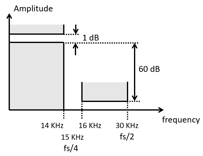
figure(3)
subplot(2,1,1)
plot(yfir(1:1024));
title('FIR lowpass output')
subplot(2,1,2)
plot(yiir(1:1024));
title('IIR lowpass output')

fvtool(Hfir);
fvtool(Hiir);

The output of both of these filters looks very similar, but it’s not identical. The most important feature is that the output of the IIR appears to loose the symmetry in the waveform. The first wiggle of the flat part of the square wave is larger than the others. The same effect does not occur in the FIR filter. In the FIR, the waveform maintains perfect symmetry. The FIR output is therefore a better reconstruction of the original input than the IIR output.

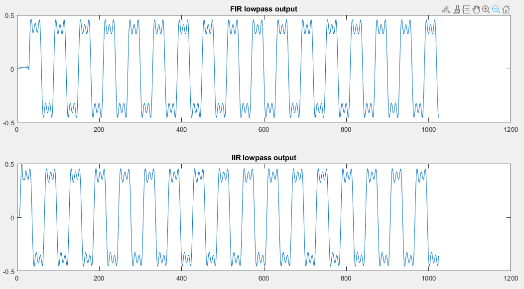
The effect becomes more pronounced when we increase the bandwidth of the modulated signal $x(t)$ . Simply doubling the base frequency of the modulated signal results in the following outputs. The IIR output has become severely distored with significant overshoot. Yet, the FIR output still maintains perfect symmetry over the square wave shape.

Linear Phase preserves the time-domain shape of a signal ¶

From these experiments, it’s clear that the FIR does a much better job at filtering a modulated signal. The IIR creates a distortion that changes the shape of the modulated waveform. This distortion is caused by the filtering process itself, and can be explained by looking at the phase response of the filter design.

From the original Fourier series, we know that the square wave requires that all harmonics are in phase. In an FIR filter, the phase response is not zero, but it is linear as a function of frequency. A linear phase response means that all frequency components are shifted uniformly in time. Indeed, assume that a frequency component at frequency $f_1$ shifts by $\phi$ .

$s(t) = sin(2 \pi f t + \phi)$

A linear phase response means that $\phi = k f$ , with $k$ a constant. Substiuting this in the earlier formula we find the following.

$s(t) & = sin(2 \pi f t + k f) \\ s(t) & = sin(2 \pi f (t + k))$

Hence, this is a sine wave that has moved in time over a delay $k$ . This move is independent of the frequency $f$ . Therefore, a complex signal with multiple harmonics will be shifted uniformly in time over all frequencies at the same time. An IIR filter does not have this advantage. In an IIR filter, the phase response is nonlinear, that is, $\phi = k f + k_2 f^2 + k_3 f^3 + ..$ . The higher order terms prevent formulating the phase shift as a simple time delay over all frequencies.

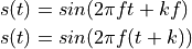
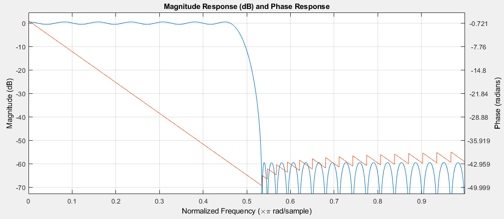
Plotting the frequency and phase response of the 60-tap FIR and the 13-tap IIR clearly shows that the IIR introduces phase distortion around the cutoff frequency. Therefore a signal $x(t)$ with a broader frequency content will be affected more profoundly.

FIR filter response (Amplitude: Blue, Phase: Orange)¶

IIR filter response (Amplitude: Blue, Phase: Orange)¶

Linear Phase in Communication¶

FIR or IIR¶

Double-side band modulation¶

Double-side band modulation of a square wave¶

DSB demodulation Lowpass filter design¶

Linear Phase preserves the time-domain shape of a signal¶