Digital Demodulation ¶

Contents

Digital Demodulation

The purpose of this lecture is as follows.

To describe DSP implementation aspects of digital demodulation
To explain the concept and purpose of adaptive filters

Demodulation is the process of restoring the data bits back from a digitally modulated signal. Last week we discussed a simple digital communication scheme called Binary Phase Shift Keying (BPSK). In BPSK, we take a stream of bits and map these bits to a stream of symbols with value -1 or +1. Next, each symbol is expanded into a pulse shape. The pulse shape is chosen such that the bandwidth required to transmit the symbol sequence is minimal, and that the symbols do not affect each other in a continuous-time symbol stream. The minimal bandwidth for a continuous-time symbol means one symbol per second per Hz of bandwidth. Next the smooth symbol stream is multiplied by a carrier.

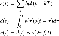
$s(t) &= \sum_k b_k \delta(t - kT) \\ d(t) &= \int_0^t s(\tau) p(t - \tau) d\tau \\ c(t) &= d(t).cos(2 \pi f_c t)$

In these equations, $s(t)$ is the symbol sequence, $d(t)$ is the pulse-shaped signal, $p(t)$ is the pulse shape, and $c(t)$ is the carrier-modulated BPSK signal.

A Raised Cosine pulse is a good choice as $p(t)$ , as it holds the middle ground between a rectangular pulse (which is limited in time, but requires extra bandwidth, much more than one Hertz per symbol per second) and a sincx pulse (strictly limited in frequency, but with a very long impulse response). The Raised Cosine filter defines an additional parameter, the rolloff-factor, which is a number between 0 and 1. A rolloff factor of 0 corresponds to a sincx pulse (filter bandwidth = symbol rate), while a rolloff factor of 1 corresponds to a filter bandwidth of twice the symbol rate.

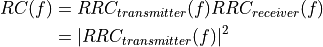
The raised cosine property is attractive because it guarantees that the symbol values do not influence each other. This distortion - if it exists - is commonly described as Inter Symbol Interference. However, the ISI-free property only holds for the Raised Cosine shape, which describes the symbol path from the transmitter all the way to the receiver. Practical transmitter/receiver chop this pulse-shaping function in two, and make use of a Root-Raised Cosine (RRC) impulse response. The square of an RRC filter (in the frequency domain) is a Raised Cosine filter. Note that the RRC filter does not hold the same ISI free property as the RC filter. Hence, an RRC-shaped waveform may still have inter symbol interference, but this symbol interference will disappear at the receiver, when it is filtered by an identical RRC filter.

$RC (f) &= RRC_{transmitter} (f) RRC_{receiver} (f) \\ &= | RRC_{transmitter} (f) | ^2$

The DSP implementation of a practical BPSK modulator requires a multi-rate pulse shaping filter. Furthermore, when the carrier frequency is a multiple of the symbol frequency, it is possible to transform the pulse shaping filter coefficients such that the pulse shaping filter implements both the pulse shaping as well as the carrier modulation. We discussed an implementation of such a BPSK modulator in matlab and in C. Lab 5 is an assignment on this BPSK modulator.

The question now is, how we can reconstruct the transmitted symbol sequence from a received continuous-time waveform. In practical implementations, the receiver and transmitter are distinct devices that operate from an independent power supply and and independent clock. The receiver only sees a continuous-time received signal. While the receiver typically knows the modulation parameters such as the carrier frequency and the pulse shape used by the transmitter, there are two parameters that are different for each communication channel and each transmission.

First, the carrier phase at the receiver is unknown. While the transmitter can generate a carrier phase of 0, the carrier phase at the receiver side depends on the latency of the signal along the channel, and the sampling phase of the analog-to-digital converter that monitors the channel.
Second, the symbol timing at the receiver is known. The receiver simply does not know when exactly the transmitter starts transmitting a new symbol. Therefore the receiver does not know exactly where the pulse shape in the received signal starts.

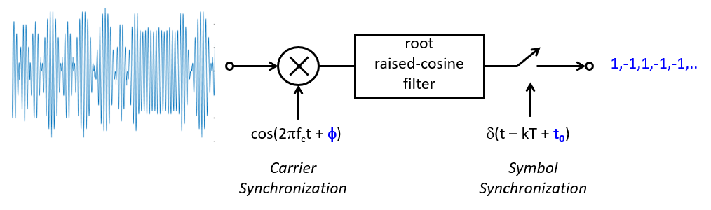
Both of these problems are addressed by the receiver, and often they are handled as seperate control loops. Using carrier synchronization, a receiver will first align its own carrier phase with that of the received signal, so that a baseband signal can be reconstructed that is similar to that of the transmitter. The baseband signal may not be identical though, due to distortions in noise in the channel. However, for proper decoding of a BPSK signal, the receiver will have to recreate the correct carrier phase.

Second, a receiver will also perform symbol synchronization, which involves determining when the output of the receiver root-raised-cosine filter contains a valid symbol. An important property – which we won’t elaborate on further – is that the best possible receiver for a given pulse shape, is a filter with an impulse reponse identical to the pulse shape. This is called the principle of matched filter reception.

In the case of our digital BPSK modulator, we have a symbol timing and a carrier phase that are linked to each other, since the carrier frequency is generated at four times the symbol frequency. This will simplify the design of a receiver, since the reconstruction of the proper carrier phase will also determine the proper symbol timing.

BPSK Demodulation using a Costas Loop ¶

John P. Costas found a technique in 1956 to decode a synchronous communication signal. He wrote a paper Synchronous Communications that explains how a carrier phase can be extracted from a received signal, thereby avoiding the need for a pilot tone (which was customary at the time). The Costas loop lies at the basis for many digital receiver techniques to this day. We will us a discrete-time version of his construction to create a BPSK receiver.

The received signal $r[n]$ is a discrete-time BPSK-modulated signal, with a carrier of fs/4 and a symbol frequency of fs/16. The received signal is downconverted into an in-phase branch and a quadrature branch by multiplying the signal with a quadrature carrier. In the following formula, $\phi[n]$ is the best estimate of the receiver regarding the carrier phase.

$x_I[n] &= r[n] . cos(n \frac{\pi}{2} + \phi[n]) \\ x_Q[n] &= r[n] . sin(n \frac{\pi}{2} + \phi[n])$

We know that $r[n]$ is a modulated signal of the following form. $s[n]$ is the discrete-time version of the pulse-shaped baseband signal. $\phi_0$ is the phase of the transmitter carrier.

$r[n] = s[n] . cos(n \frac{\pi}{2} + \phi_0)$

Thus $x_I[n]$ and $x_Q[n]$ are double-sideband signals:

$x_I[n] &= s[n] . cos(n \frac{\pi}{2} + \phi_0) . cos(n \frac{\pi}{2} + \phi[n]) \\ x_Q[n] &= s[n] . cos(n \frac{\pi}{2} + \phi_0) . sin(n \frac{\pi}{2} + \phi[n])$

Using

$cos A . cos B &= \frac{cos(A+B) + cos(A-B)}{2} \\ cos A . sin B &= \frac{sin(A+B) - sin(A-B)}{2} \\$

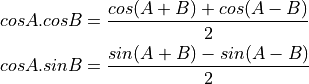
We expand the high and low frequencies in each of $x_I[n]$ and $x_Q[n]$ .

$x_I[n] &= s[n] . \frac{(cos(n \pi + \phi_0 + \phi[n]) + cos(\phi_0 - \phi[n]))}{2} \\ x_Q[n] &= s[n] . \frac{(sin(n \pi + \phi_0 + \phi[n]) - sin(\phi_0 - \phi[n]))}{2}$

Both of these branches are filtered with a matched filter. The lowpass nature of this filter will remove the high-frequency components in each of $x_I[n]$ and $x_Q[n]$ , and we are left with the filtered outputs:

$y_I[n] &= s[n] . cos(\phi_0 - \phi[n]) = s[n] . cos(\phi_{err})\\ y_Q[n] &= s[n] . (- sin(\phi_0 - \phi[n])) = s[n] . (-sin(\phi_{err}))$

Assume for a moment that $\phi_0 = \phi[n]$ , then it follows that $z_I[n] = s[n]$ . Thus, when the Costas loop is synchronized, the demodulated signal can be found directly at the output of the I-branch filter!

However, until the loop is synchronized, we will keep on computing a phase error.

$e[n] &= - s^2[n] cos(\phi_{err}) sin(\phi_{err}) \\ &= - s^2[n] \frac{sin(2 \phi_{err})}{2}$

$s^2[n]$ is always positive, so the sign of $e[n]$ is completely determined by $\phi_{err}$ . When the error is small, then the error signal can be used as a negative feedback signal. Thus, the error signal is used to adjust $\phi[n]$ as follows. $k$ is a small loop constant, such as 0.05.

$\phi[n] = \phi[n-1] + k . e[n]$

Thus, we conclude that this remarkable structure is capable of demodulating a synchronously modulated BPSK signal, and when the carrier phase is unknown, the structure can extract it from the received symbols.

Matlab Design ¶

The following matlab code illustrates the implementation of a BPSK demodulator using a Costas loop. First, we have to create a BPSK modulated signal. This is straightforward, and it relies on code that we discussed in previous lecture.

% COSTAS LOOP demo

%--------------------------------------------
% BPSK modulator

samplespersymbol = 16;      % simulation done at this number of samples per symbol
numsymbols       = 200;      % simulate this number of symbol
carrierfreq      = 4;       % times the symbol frequency; <= samplespersymbol

carriersync      = [ 1  1  1  1  1  1  1  1  1  1  1  1  1  1  1 ];
symbolsync       = [ 1 -1  1 -1  1 -1  1 -1  1 -1  1 -1  1 -1  1 ];

sync1    = [carriersync symbolsync];
payload  = (floor((rand(numsymbols-length(sync1),1) * 2)) - 0.5) * 2;
symbols  = [sync1'  ; payload]; %'

offset   = pi / 16;
carrier  = cos(offset + 2 * pi *    carrierfreq*((1:samplespersymbol)-1)/samplespersymbol);

fullcarrier      = repmat(carrier', numsymbols, 1);     % '
rcpulse          = rcosdesign(0.25, 3, samplespersymbol, 'sqrt');
rcupsym          = conv(upsample(symbols, samplespersymbol), rcpulse);
modrcsym         = fullcarrier .* rcupsym(1:(samplespersymbol*numsymbols));

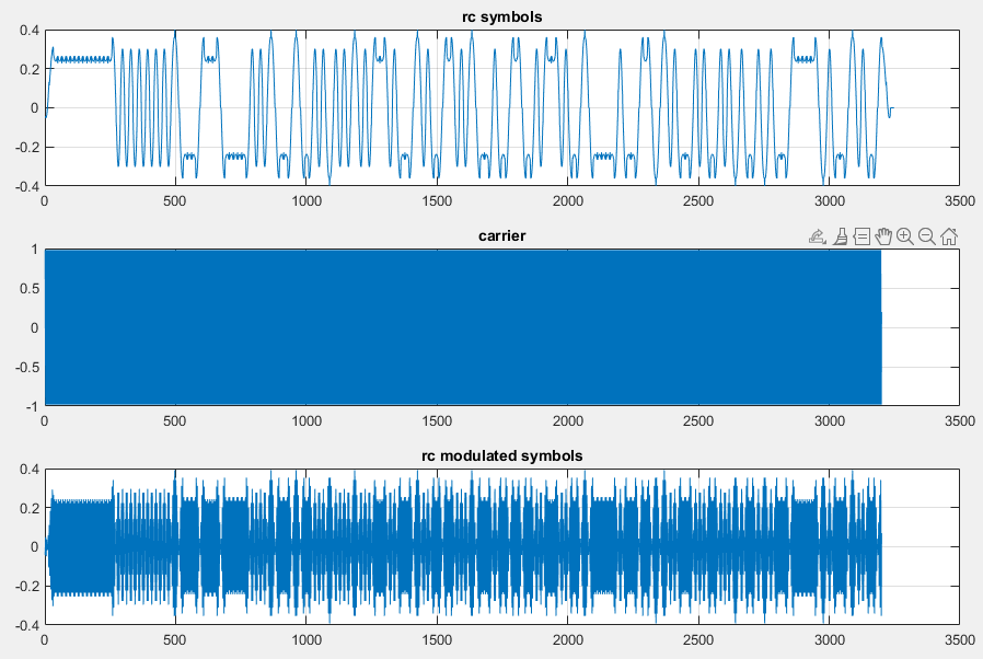
figure(1)
pwelch(modrcsym);

figure(2)
subplot(3,1,1);
hold off
plot(rcupsym);
grid
title('rc symbols');
subplot(3,1,2);
plot(fullcarrier);
title('carrier');
grid
subplot(3,1,3);
plot(modrcsym);
title('rc modulated symbols');
grid

This code allows the user to specify a carrier phase offset, thereby simulating a transmitter with a different carrier phase. The sequence at the start of the transmission is a so-called training sequence. It’s a sequence with known symbols, which help with calibration and syncrhonization at the receiver side.

Next, we simulate the receiver using a Costas loop.

%--------------------------------------------
% BPSK demodulator
% adapted from: https://dsp.stackexchange.com/questions/22316/simulating-bpsk-costas-loop-in-matlab

rfsignal = modrcsym;
phi      = zeros(length(rfsignal),1);
xi       = zeros(length(rfsignal),1);
xq       = zeros(length(rfsignal),1);

% costas loop
for i = 2:length(rfsignal)
  xi(i)    = rfsignal(i) .* cos(- 2 * pi * i * carrierfreq / samplespersymbol - phi(i-1));
  xq(i)    = rfsignal(i) .* sin(- 2 * pi * i * carrierfreq / samplespersymbol - phi(i-1));
  zi       = conv(rcpulse, xi(1:i));
  zq       = conv(rcpulse, xq(1:i));
  error(i) = zi(i) * zq(i);
  phi(i)   = phi(i-1) + 0.1 * error(i);
end

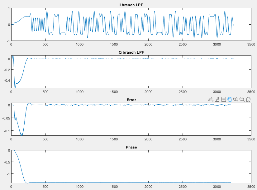
figure(3)
subplot(4,1,1)
plot(zi)
title('I branch LPF')
subplot(4,1,2)
plot(zq)
title('Q branch LPF')
subplot(4,1,3)
plot(error)
title('Error')
subplot(4,1,4)
plot(phi)
title('Phase')

The I-branch output is almost zero, because the BPSK signal only contains an in-phase component. The Q-branch output clearly shows the demodulated signal which appears almost identical to the transmitted baseband signal.

C Design ¶

The design of a Costas loop in C, as a DSP program, is less amendable to optimization tricks such as multirate expansion and filter coefficient optimization. This is because we have to be able to compute with an arbitrary carrier phase and an arbitrary symbol timing. Furthermore, we are facing potentially complex trigonometric computations in order to compute the sine and cosine of an arbitrary phase. The following C code illustrates a Costas loop receiver for a transmitter with a carrier at 2 KHz (4 samples per symbol, 8000 samples per second). Note in particular the use of the arm_cos_f32 and arm_sin_f32 functions, which are functions from the ARM CMSIS DSP library for fast computation of sine and cosine.

#include "xlaudio.h"

#define SYMBOLS 3
#define UPSAMPLE 16

#define NUMCOEF (SYMBOLS * UPSAMPLE + 1)

float32_t coef[NUMCOEF] = {
  -0.042923315, -0.047711509,   -0.050726122, -0.05161785,
  -0.050086476, -0.045895194,   -0.038883134, -0.02897551,
  -0.016190898, -0.00064525557,  0.017447588,  0.037779089,
   0.05995279,   0.083494586,    0.10786616,   0.13248111,
   0.1567233,    0.17996659,     0.20159548,   0.22102564,
   0.23772369,   0.2512255,      0.26115217,   0.26722319,
   0.26926623,   0.26722319,     0.26115217,   0.2512255,
   0.23772369,   0.22102564,     0.20159548,   0.17996659,
   0.1567233,    0.13248111,     0.10786616,   0.083494586,
   0.05995279,   0.037779089,    0.017447588, -0.00064525557,
  -0.016190898, -0.02897551,    -0.038883134, -0.045895194,
  -0.050086476, -0.05161785,    -0.050726122, -0.047711509,
  -0.042923315
};

float32_t qtaps[NUMCOEF];
float32_t itaps[NUMCOEF];
float32_t phi = 0.0;

float32_t filter(float32_t input) {
    uint32_t i;

    float32_t qresult = 0.0;
    float32_t iresult = 0.0;

    static unsigned carrier = 0;
    carrier = (carrier + 1) & 3; // carrier = fs/4

    itaps[0] = input * arm_cos_f32(carrier * M_PI /2.0 + phi);
    qtaps[0] = input * arm_sin_f32(carrier * M_PI /2.0 + phi);

    for (i = 0; i< NUMCOEF; i++) {
        qresult += qtaps[i] * coef[i];
        iresult += itaps[i] * coef[i];
    }

    for (i = NUMCOEF-1; i>0; i--) {
        qtaps[i] = qtaps[i-1];
        itaps[i] = itaps[i-1];
    }

    float32_t error = qresult * iresult;
    phi = phi + 0.1 * error;

    if (xlaudio_pushButtonRightDown())
        return error;

    if (xlaudio_pushButtonLeftDown())
        return input;

    return iresult;
}

uint16_t processSample(uint16_t x) {
    float32_t input = xlaudio_adc14_to_f32(x);
    return xlaudio_f32_to_dac14(filter(input));
}

#include <stdio.h>

int main(void) {
    WDT_A_hold(WDT_A_BASE);

 //   xlaudio_init_intr(FS_8000_HZ, XLAUDIO_MIC_IN, processSample);
    xlaudio_init_intr(FS_8000_HZ, XLAUDIO_J1_2_IN, processSample);

    int c = xlaudio_measurePerfSample(processSample);
    printf("Cycles %d\n", c);

    xlaudio_run();
    return 1;
}

When Synchronization alone is not enough ¶

So far, we have constructed a receiver that is able to identify the unknown carrier phase and the unknown timing of a modulated signal. However, the real channel environment is quite complex, and can cause many different effects on a modulated signal.

The channel will add noise, and that is to be expected. Noise is fine, as we know (or have accepted) from theory that the matched-filter receiver gives us the best possible receiver for noise signals.
The channel may cause frequency-dependent amplitude distortion. For example, high frequencies may be attenuated differently than low frequencies. This may occur, for example, when wireless signals propagated through different paths, then attenuation may occur due to so-called multi-path effects.
The channel may cause non-linear phase distortion. For example, cable modems use the cable network for communications. This network is designed to be an allpass network (at the carrier frequencies of the transmissions), by this allphass network can still suffer nonlinear phase distortion.

Both phase and frequency distortion are problematic for a synchronous receiver, because its principle of operation relies on a predictable pulse shape. The solution to this distortion is to adapt the receiver characteristic to the channel using an additional filter, the equalizer. The equalizer is programmed to the inverse characteristic of the channel, thereby restoring the allpass amplitude response and the linear phase response.

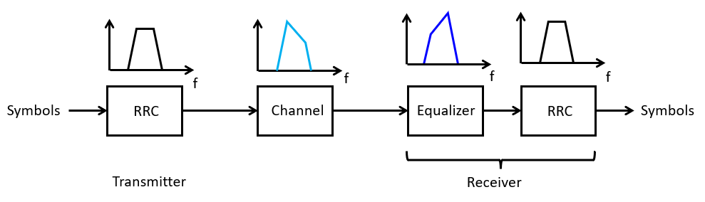
The problem is then, how the coefficients of the equalizer filter can be found, when the channel may not be known beforehand? Amazingly, a class of filters known as adaptive filters are designed to solve precisely that problem: remove a distortion from a signal be means of a filter with adaptive coefficients. In the following, we describe the basic operation of an adaptive filter.

Basic Adaptive Filter ¶

An adaptive FIR filter accepts an input signal x and produces an output signal y. The FIR coefficients of this filter are adjustable, meaning that at every new sample of x, the coefficients can take on a new value. The new value of filter coefficients is determined using a coefficient update algorithm, which computes an adjustment for each filter coefficient based on an error signal e. The error signal e is typically computed as the difference between the actual output signal y and a desired output signal d.

The desired output signal d depends on the specific application of the adaptive filter. However, the adaptive algorithm will change the coefficients so as to minimize the mean squared value of the error signal e. That is, given that the filter output is defined by filter coefficients $\boldsymbol{w(n)} = [w_0(n) w_1(n) .. w_{N-1}(n)]^T$ , we try to minimize the expected square error:

$\min_{\boldsymbol{w}(n)} E[ e^2(n)]$

Equalization ¶

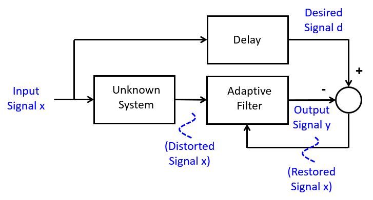
While there are many different applications for the adaptive filter, we will focus specifically on the equalization problem. In equalization, we are using an adaptive filter to remove (linear) distortions from a received signal. This is a common problem in data communictions, when signals are distored by a non-allpass communications channel. The adaptive filter creates an inverse response to the distortion, using a delayed version of the correct input signal $x$ , in order to restore the received signal to its original form.

You may wonder how such a delayed version of $x$ can be transmitted, when it’s not possible to transmit the real-time version $x$ . The answer is that this delayed $x$ does not have to be identical to the real-time $x$ . In other words, the equalizer can first go through a training phase, during which the coefficients are adapted in order to match the characteristics of the communications channel. Next, the adaptive filter coefficients are fixed, and the real-time $x$ transmission can start.

A well-known example of an equalizer training sequence can be heard in the startup sequence of an voiceband modem. While voiceband modems are largely a thing of the past now, this youtube link gives you an idea how that sounded like.

Computing the Equalizer Coefficients ¶

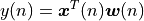
An adaptive filter implemented as an FIR with N taps and weights $\boldsymbol{w}(n) = [w_0(n) w_1(n) .. w_{N-1}(n)]^T$ filters input samples $\boldsymbol{x}(n) = [x_0(n) x_1(n) .. x_{N-1}(n)]^T$ . At the nth sample instant, the output of the filter is given by the dot product of $\boldsymbol{w}(n)$ and $\boldsymbol{x}(n)$ :

$y(n) = \boldsymbol{x}^T(n) \boldsymbol{w}(n)$

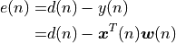
The instantaneous error at the nth sample instant is given by the difference of $d(n)$ and $y(n)$ .

$e(n) =& d(n) - y(n) \\ =& d(n) - \boldsymbol{x}^T(n) \boldsymbol{w}(n)$

The instantaneous squared error signal is given by:

$e^2(n) = d^2(n) - 2d(n) \boldsymbol{x}^T(n) \boldsymbol{w}(n) + \boldsymbol{w}^T(n) \boldsymbol{x}(n) \boldsymbol{x}^T(n) \boldsymbol{w}(n)$

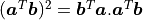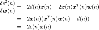
Note that we make use of the property $(\boldsymbol{a}^T \boldsymbol{b})^2 = \boldsymbol{b}^T \boldsymbol{a} . \boldsymbol{a}^T \boldsymbol{b}$ .

We are interested in minimizing the expected value of the squared error signal, and we will do this by making changes to the filter weights $\boldsymbol{w}(n)$ . Hence, we differentiate the expression for $e^2(n)$ with respect to $\boldsymbol{w}(n)$ and look for a minimum.

$\frac{\delta e^2(n)}{\delta \boldsymbol{w}(n)} &= - 2d(n) \boldsymbol{x}(n) + 2 \boldsymbol{x}(n) \boldsymbol{x}^T(n) \boldsymbol{w}(n) \\ &= -2 \boldsymbol{x}(n) (\boldsymbol{x}^T(n) \boldsymbol{w}(n) - d(n)) \\ &= -2 e(n) \boldsymbol{x}(n)$

An iterative version of this algorithm will therefore use the value of this derivative to decide on how to adjust the coefficients. A well known strategy is steepest decent, which means that you’ll make a change which is a fraction of the derivative at the point where the derivative is computed. In other words, you compute the coefficient series as follows. In this formula, $\beta$ is a constant much smaller then 1.

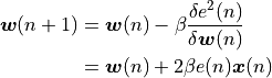
$\boldsymbol{w}(n + 1) &= \boldsymbol{w}(n) - \beta \frac{\delta e^2(n)}{\delta \boldsymbol{w}(n)} \\ &= \boldsymbol{w}(n) + 2 \beta e(n) \boldsymbol{x}(n)$

The Least Mean Squares (or LMS) filtering algorithm is an adaptive FIR where coefficients are adjusted according to an error signal $e(n)$ as in the previous formula.

Conclusions ¶

We discusssed on important construction to demodulation synchronous data communications - the Costas Loop. Using the Costas loop, we are able to recover the carrier phase. When used in a digital modulation scheme where the symbol rate and carrier frequency are coupled, recovery of the carrier phase also yields the symbol timing - even though we will need to choose which of n samples (at n samples per symbol) is the through symbol peak.

In addition, we discussed that the channel may act as a filter of its own, adding additional amplitude and phase distortion. This distortion has to be removed before demodulation through channel equalization. An adaptive filter can automatically estimate the channel characteristic and remove channel distortion.

This concludes our whirlwind tour through the use of DSP in data communications. Data communications is a sprawling research topic at the forefront of research and development. Dig further into this material for example through Digital Communications by Bernard Sklar and Fredric Harris, or Digital Communications by John Proakis.