IIR Implementation Techniques
The purpose of this lecture is as follows.
To describe the direct-form I and direct-form II implementations of IIR designs
To describe the cascade-form implementations of IIR designs
To describe transpose-form implementations of IIR designs
To describe parallel-form implementations of IIR designs
To study the design of IIR filters using the bilinear transformation
To demonstrate useful functions in Matlab used for polynomial manipulation
Attention
The sample code for this lecture is on this github repository
Direct-form IIR implementation
An IIR filter is a digital filter described by the following input/output relationship
![y[n] = \sum_{k=0}^{M} b[k] x[n-k] - \sum_{k=1}^{N} a[k] y[n-k]](_images/math/8914117dac863edf6bdbb535dbc39ccd49c86aab.png)
which means that the output of an IIR filter is defined by both the previous inputs as well as the previous outputs.
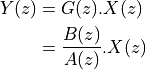
We can write this equivalently as a z-transform
![Y(z) = X(z) . \sum_{k=0}^{M} b[k] z^{-k} - Y(z) . \sum_{k=1}^{N} a[k] z^{-k}](_images/math/881eaa935dc9c1e8d9963d0fef97f4494b35d8f1.png)
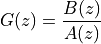
Assume that the order of the numerator and denominator are identical, then we can write the filter transfer function as follows.
![G(z) =& \frac{Y(z)}{X(z)} \\
G(z) =& \frac{\sum_{k=0}^{N} b[k] z^{-k}}{ 1 + \sum_{k=1}^{N} a[k] z^{-k}}](_images/math/22e93a213423149603f0f5b1c8616a95fd5b16f7.png)
Since these are N-th order polynomials in z, they contribute N zeroes and N poles. For an IIR system to be causal and stable, all poles must lie within the unit circle.
We can find the locations of the zeroes and poles of an arbitrary  by
multiplying the numerator and denominator by
by
multiplying the numerator and denominator by  and finding the roots
of each polynomial. See further for an example on using Matlab to find these roots.
and finding the roots
of each polynomial. See further for an example on using Matlab to find these roots.
Direct-form I IIR Implementation
If we consider a transfer function of the form
and we look for the output signal  in response to the input signal
  , then we compute:
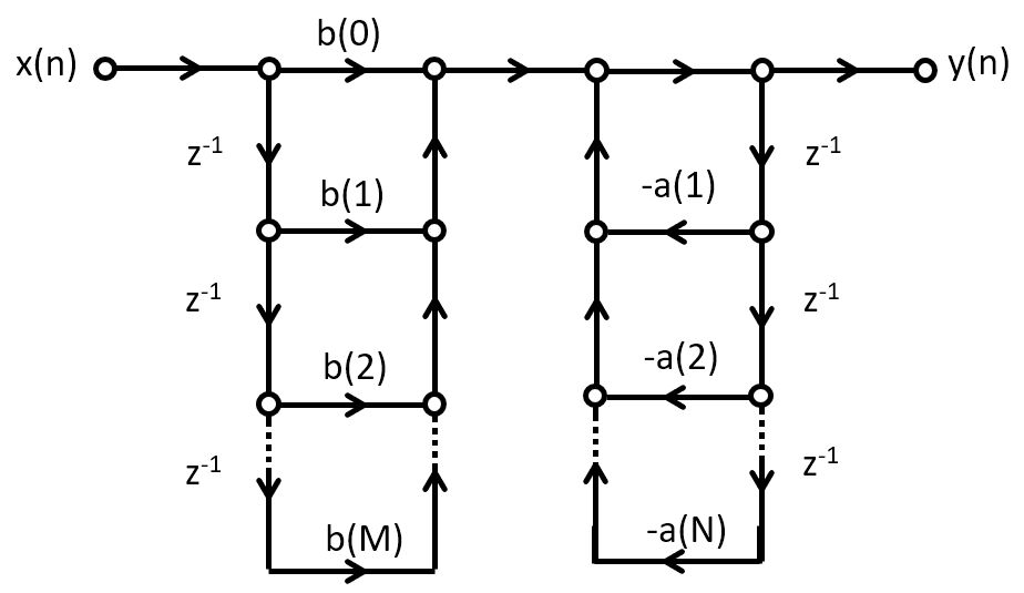
A direct-form I IIR implementation first computes the zeroes, and then the poles:
![Y(z) &= \frac{1}{A(z)}.[B(z).X(z)]](_images/math/07f0627091b961291099f1454db5ed97b2d8e017.png)
In the time domain we would implement
![w(n) &= \sum_{k=0}^{M} b[k] x[n-k] \\
y(n) &= w(n) - \sum_{k=1}^{N} a[l] y[n-l]](_images/math/f0af09e5f310fa289bd0e7c762dedb8da455062e.png)
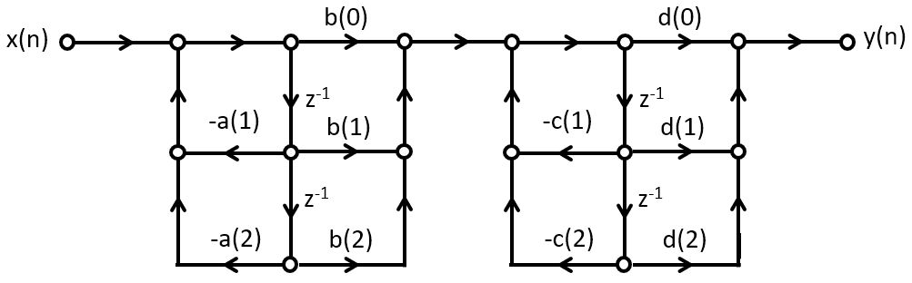
This formulation leads to a design as shown below. This design requires
 multiplications per output sample,
 additions per output sample,
and delays.
additions per output sample,
and delays.
Direct-form II IIR Implementation
A direct-form II IIR implementation first computes the poles, and then the zeroes:
![Y(z) &= B(z) . [\frac{1}{A(z)}.X(z)]](_images/math/703a138a01492572c98c1dbaed91422d85e44dbf.png)
This structure is created by swapping the order of the operations in a direct-form I structure. However, an important optimization is possible because the taps can be shared by the feedback part as well as by the feedforward part.
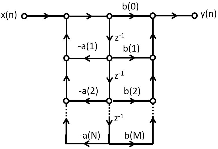
This design requires multiplications per output sample,
additions per output sample,
and  delays.
This implementation has the mimimum number of delays possible for a given transfer function. Hence, an N-th order FIR, and an N-th order IIR, both can be implemented with only N delays.
Cascade IIR Implementation
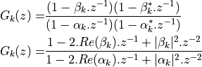
Just as with the FIR implementation, a cascade IIR is created by factoring the
nominator and denominator polynomials in . Assuming both
nominator and denominator have order N, then
![G(z) =& \frac{\sum_{k=0}^{N} b[k] z^{-k}}{ 1 + \sum_{k=1}^{N} a[k] z^{-k}} \\
=& A . \prod_{k=1}^{N} \frac{1 - \beta_k . z^{-1}}{1 - \alpha_k . z^{-1}}](_images/math/fa486767a8d82ea80bfce4df0032c0902d29ca25.png)
It’s common to formulate this as second-order sections, in order to ensure that complex (conjugate) poles and complex (conjugate) zeroes can be represented with real coefficients. Each such a section contains a conjugate pole pair and/or conjugate zero pair.
Cascade IIR Example
We implement the following cascade IIR design in C.
It has four poles, located at  , as well
as three zeroes, located at
, as well
as three zeroes, located at  .
.
The first step is to derive the proper filter coefficients. We group the poles and zeroes as follows.
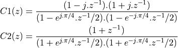
Which can be multiplied out to derive the filter coefficients:
The construction of the filter proceeds similar to the cascade FIR filter. First, we create a data structure for the cascade IIR stage, containing filter coefficients and filter state. We will use a direct-form Type II design, which gives us a state of only two variables.
 1typedef struct cascadestate {
 2    float32_t s[2];   // state
 3    float32_t b[3];  // nominator coeff  b0 b1 b2
 4    float32_t a[2];  // denominator coeff   a1 a2
 5} cascadestate_t;
 6
 7float32_t cascadeiir(float32_t x, cascadestate_t *p) {
 8    float32_t v = x - (p->s[0] * p->a[0]) -  (p->s[1] * p->a[1]);
 9    float32_t y = (v * p->b[0]) + (p->s[0] * p->b[1]) + (p->s[1] * p->b[2]);
10    p->s[1] = p->s[0];
11    p->s[0] = v;
12    return y;
13}
14
15void createcascade(float32_t b0,
16                   float32_t b1,
17                   float32_t b2,
18                   float32_t a1,
19                   float32_t a2,
20                   cascadestate_t *p) {
21    p->b[0] = b0;
22    p->b[1] = b1;
23    p->b[2] = b2;
24    p->a[0] = a1;
25    p->a[1] = a2;
26    p->s[0] = p->s[1] = 0.0f;
27}
The cascadestate_t now contains both feed-forward and feed-back coefficients.
The cascadeiir function is likely the most complicated element
for this design. The order of evaluation of each expression is chosen
so that we don’t update filter state until it has been used for all expressions
required. In cascadeiir we first compute the intermediate variable v which
corresponds to the center-tap of the filter. Next, we compute the
feed-forward part based in this intermediate v. Finally, we update the filter
state and return the filter output y.
The filter program then consists of filter initialization, followed by the chaining of filter cascades:
 1cascadestate_t stage1;
 2cascadestate_t stage2;
 3
 4void initcascade() {
 5    createcascade(  /* b0 */  1.0f,
 6                    /* b1 */  0.0f,
 7                    /* b2 */  1.0f,
 8                    /* a1 */ -0.7071f,
 9                    /* a2 */ 0.25f,
10                    &stage1);
11    createcascade(  /* b0 */  1.0f,
12                    /* b1 */  1.0f,
13                    /* b2 */  0.0f,
14                    /* a1 */ +0.7071f,
15                    /* a2 */ 0.25f,
16                    &stage2);
17}
18
19uint16_t processCascade(uint16_t x) {
20
21    float32_t input = xlaudio_adc14_to_f32(0x1800 + rand() % 0x1000);
22    float32_t v;
23
24    v = cascadeiir(input, &stage1);
25    v = cascadeiir(v, &stage2);
26
27    return xlaudio_f32_to_dac14(v*0.125);
28}
Transposed Structures
The transposition theorem says that the input-output properties of a network remain unchanged after the following sequence of transformations:
Reverse the direction of all branches
Change branch points into summing nodes and summing nodes into branch points
Interchange the input and output
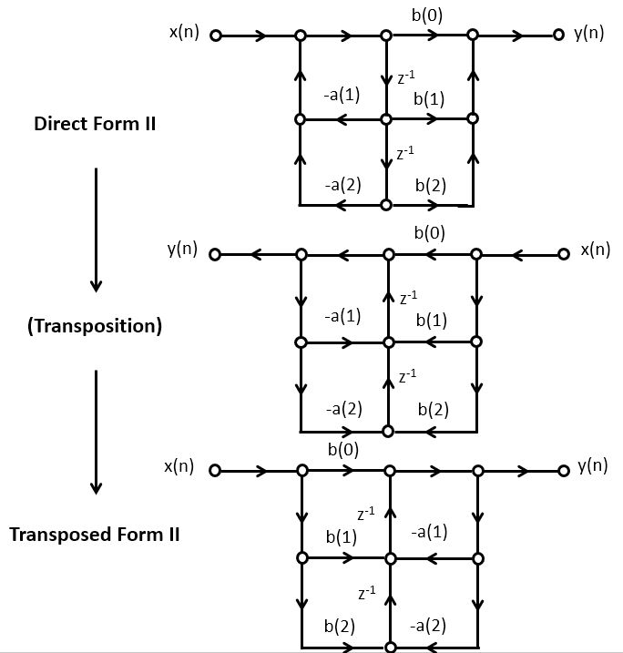
Once you have the defined the transposed-form structure, you can develop a C program for that implementation. The transposed-form IIR can be implemented using the same data structure as the direct-form IIR; only the filter operation would be rewritten. The following is the implementation of a second-order section of a transposed direct-form II design.
 1typedef struct cascadestate {
 2    float32_t s[2];   // state
 3    float32_t b[3];  // nominator coeff  b0 b1 b2
 4    float32_t a[2];  // denominator coeff   a1 a2
 5} cascadestate_t;
 6
 7float32_t cascadeiir_transpose(float32_t x, cascadestate_t *p) {
 8    float32_t y = (x * p->b[0]) + p->s[0];
 9    p->s[0]     = (x * p->b[1]) - (y * p->a[0]) + p->s[1];
10    p->s[1]     = (x * p->b[2]) - (y * p->a[1]);
11    return y;
12}
Parallel Structures
IIR filters are rarely implemented as single, monolithic structures; the risk for instability is too high. One way to achieve this, is to use a cascade expansion of an IIR filter.
An alternate implementation is the parallel-form implementation. The idea of a parallel-from implementation is to build two or more parallel filters, that can be summed up together to form the overall transfer function.
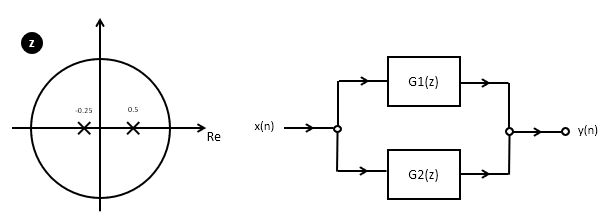
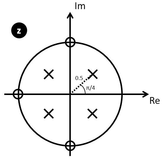
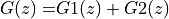
Let’s consider this for the pole plot shown in the figure. This design has two poles, so it’s transfer function would be:
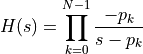
To build a parallel design, we have to decompose
The design of these partial function proceeds by partial fraction expansion.
We split the poles of the overall function in two.
In this case, one pole goes with  and the other pole goes with
 . Partial fraction expansion will now proceed by looking for terms
A and B such that:
. Partial fraction expansion will now proceed by looking for terms
A and B such that:

Solving for A and B we find:
The meaning of  is that a second order system can be implemented by
two independent first-order systems, whose output is added together.
is that a second order system can be implemented by
two independent first-order systems, whose output is added together.
Design of Butterworth IIR using Bilinear Transformation
For historical reasons, many common IIR filter structures are based on analog filter designs. Often, these analog filters have a solid theoretical foundation and properties, which makes them also attractive for digital implementation. Of course, a digital filter is band-limited to half of the sampling frequency, so a digital filter has to approximate the response of the analog filter by mapping the response over an infinite frequency band into an equivalent response over a finite frequency band. We will illustrate these ideas using one concrete filter design called the Butterworth filter, and one frequency mapping method called the bilinear transformation.
A Butterworth filter is an analog filter defined by the magnitude of its Fourier transform:
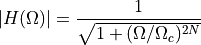
The filter is defined by two parameters: the filter order  and the cutoff frequency
  . The Butterworth filter is also called a maximally flat filter, meaning that its frequency response in the passband is almost perfectly flat. Of course, almost is not completely; for any small increase of
  ,
,  will decrease. A Butterworth filter is therefore also called a monotonic filter: you will never see any ‘wiggles’ in either the passband nor stopband of a Butterworth filter.
At the cutoff frequency , the response of the butterworth filter is 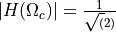 , meaning that the output power of the filter at that frequency will be half of the input power. The response of the butterworth filter at the cutoff frequency in dB is
 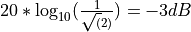 .
.
When you design a practical lowpass filter, the specifications may not come as a cutoff frequency and filter order, but rather as a passband frequency  , stopband frequency
  , passband response
  and stopband response
  .
.
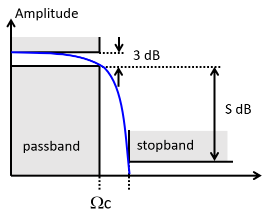
One can show that for a given , , and , the filter order N is constrained as follows.
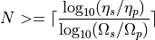
where  , the stopband ripple, and
  , the passband ripple. Furthermore, the cutoff frequency of the Butterworth filter that works with the given passband and stopband is given by
A typical filter design program therefore asks for the filter specifications, and then computes the required filter order to match these specifications.
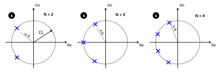
An interesting property of the Butterworth filter is that its poles are symmetrically distributed on a half circle in the s-plane:
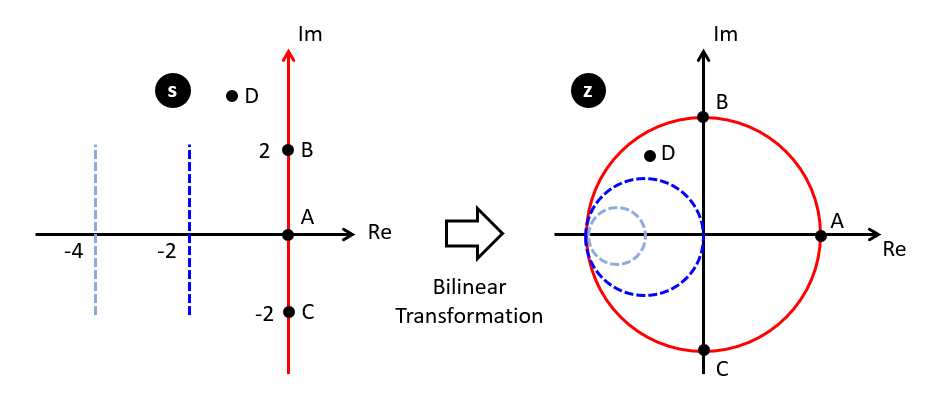
From a given analog filter (with a specification given in the s-plane), we would like to determine an equivalent discrete-time implementation. This requires one to map the s-plane into the z-plane, or conversely a continuous-time impulse response (potentially infinite in length) to a discrete-time impulse response. There are several techniques that achieve such a transformation, and we will discuss one of them known as the bilinear transformation.
The bilinear transformation defines a relation between the Laplace s-variable and the Z-transform z-variable as follows.
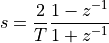
The bilinear transformation maps the entire right-half plane of the Laplace domain into the unit circle of the z-transform. The frequency from DC to infinite is mapped along the unit circle, such that the point at z = -1 maps to s =  .
.
The ability to transform the z variable into the s variable, allows a designer to create the digital equivalent of an analog (s-domain) filter, by substituting the s-variable to a z-variable (and by mapping poles from the s-plane to the z-plain). This leads to the following bilinear filter design procedure for a digital filter:
Specify the filter characteristic in the digital domain, including passband and stopband frequencies, as well as passband and stopband ripple.
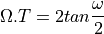
Find the equivalent analog filter characteristic by prewarping the digital frequencies to analog frequencies. This prewarping makes use of the bilinear relation that links the continuous-time analog frequency
to the discrete-time digital frequency  , with sample period
  :
:
Use an analog filter design procedure to find
 . For example, in the case of Butterworth filter design, we use the passband and stopband specification in the continuous time domain to find the required filter order , and the location of the poles.
Compute the digital equivalent filter using the bilinear transformation, by substituting
 with
with  .
.
Butterworth Design Example
Consider the following design example of a Butterworth lowpass filter, with passband at  and stopband at
  , passband response
  and stopband response
  .
.
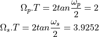
First, we prewarp the digital frequencies into analog frequencies:
We also compute the equivalent passband ripple and stopband ripple:
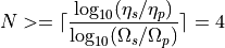
These four factors are used to determine the minumum order of the required Butterworth filter:
as well as the cutoff frequency:
The 4 poles are located in the s-plane on a circle with radius at  . This leads to :
To obtain  , we substitute s in this equation with the bilinear transformation for
  :
:

This leads to the nominator and denominator polynomials in . The following Matlab program shows the computation of these polynomials.
wp = 0.5 * pi
ws = 0.7 * pi
dp = -3
ds = -20
WpT = 2 * tan(wp / 2)
WsT = 2 * tan(ws / 2)
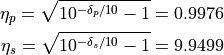
ep = sqrt(10^-(dp/10)-1)
es = sqrt(10^-(ds/10)-1)
N = ceil(log10(es/ep) / log10(WsT / WpT))
WcT = WpT * ep^(-1/N)
k = 0:N-1
pkT = WcT * exp(1j*pi*(2*k+N+1)/2/N)
b = real(prod(pkT ./ (pkT-2))) * poly(-ones(1,N))
a = real(poly((2+pkT)./(2-pkT)))
This leads to the following output:
b =

    0.0941    0.3764    0.5646    0.3764    0.0941


a =

    1.0000    0.0015    0.4860    0.0003    0.0177
From which we conclude that the required discrete-time Butterworth filter has the following transfer function:

As we discussed above, the direct form is not used for high-order IIR implementations. Instead, is broken down into second-order sections. Matlab has a function for this called tf2sos (transfer function to second-order-sections).
tf2sos(b,a)
ans =
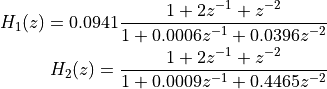
0.0941 0.1882 0.0941 1.0000 0.0006 0.0396
1.0000 2.0000 1.0000 1.0000 0.0009 0.4465
This yields two second-order sections, namely:
Using Matlab
Designing Filters
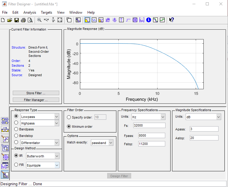
The Butterworth lowpass filter designed earlier can be created directly in Matlab using filterDesigner. As an example, we create the same filter using a samplefrquency of 32 Khz.
At this sample frequency, the passpand frequency is 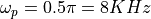 , the stopband frequency is
  . In addition, the passband response is -3dB and the stopband response is -20dB. The resulting filter is a fourth-order filter, as expected:
Matlab can also generate the filtercoefficients for a cascade implementation. Using ‘Targets->Generate C Coefs’, we obtain the following file. The format is somewhat redundant, but contains essentially the same coefficients as we have derived above; internally, Matlab filterDesigner also uses a bilinear transformation to design a discrete-time Butterworth filter. Hence, we can expect to find the same coefficients as we derived earlier.
#define MWSPT_NSEC 5
const int NL[MWSPT_NSEC] = { 1,3,1,3,1 };
const real32_T NUM[MWSPT_NSEC][3] = {
  {
     // K0
     0.3618303537,              0,              0
  },
  {
     //       b00             b01              b02
                1,              2,              1
  },
  {
    // K1
     0.2600458264,              0,              0
  },
  {
    //         b10             b11             b12
                1,              2,              1
  },
  {
                1,              0,              0
  }
};
const int DL[MWSPT_NSEC] = { 1,3,1,3,1 };
const real32_T DEN[MWSPT_NSEC][3] = {
  {
                1,              0,              0
  },
  {
     //       a00             a01              a02
                1, 0.000858646119,   0.4464627504
  },
  {
                1,              0,              0
  },
  {
     //       a10             a11              a12
                1,0.0006171050481,  0.03956621885
  },
  {
                1,              0,              0
  }
};
Marking the coefficients b00, b01, … as shown in the code, the filter coefficients are now mapped as follows from this C header file:
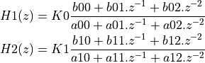
Note that K0.K1 = 0.0941, the same amplification constant we have derived before. Furthermore, note how each of a00, a01, a02, a10, a11, a12 are the same as the coefficients we computed manually in the previous section.
Finding Poles and Zeroes
Attention
To identify pole and zero locations, use the roots function in Matlab,
which finds the roots of a polynomial. For a polynomial
 ,
the roots can be found through
,
the roots can be found through roots([a0 a1 ... an])
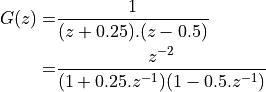
Example: Find the zeroes and poles of
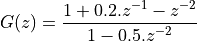
The roots function in Matlab will return the locations of zeroes and poles:
>> roots([1 0.2 -1])  % numerator coefficients

ans =

   -1.1050
    0.9050

>> roots([1 0 -0.5])  % denominator coefficients

ans =

    0.7071
   -0.7071

>> zplane([1 0.2 -1],[1 0 -0.5])  % create a pole-zero plot
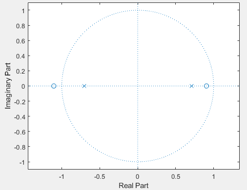
We can write G(z) in factored form as follows
![G(z) =& \frac{(1 - n_0 . z^{-1})(1 - n_1 . z^{-1})}{(1 - p_0 . z^{-1})(1 - p_1 . z^{-1}])} \\
G(z) =& \frac{(1 + 1.1050.z^{-1})(1 - 0.9050.z^{-1})}{(1 + 0.7071.z^{-1})(1 - 0.7071.z^{-1})}](_images/math/e67e5932e1c563a4fa1413b5b8f32c6f603bb4ad.png)
Finding Partial Fraction Expensions
Attention
To perform partial fraction expansion, use the residue function in Matlab.
For a transfer function 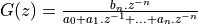 the partial fraction is found as
 [r,p,k] = residue([0 0 ... bn], [a0 a1 .. an]).
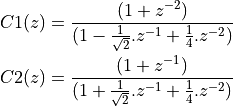
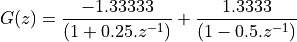
The parallel form of an IIR requires partial fraction expansion. Consider the following example, where the objective is to find A and B:
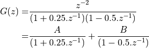
>> % compute G(z)
>> a = conv([1 0.25],[1 -0.5])

a =

   1.0000   -0.2500   -0.1250

% In other words, G(z) = z^-2 / (1 - 0.25.z^-1 - 0.125.z^-2)

>> % compute terms A and B using 'residue'
>> [r,p,k] = residue([0 0 1],a)

r =

    1.3333
   -1.3333


p =

    0.5000
   -0.2500


k =

     []
From the r term in the Matlab output, we conclude that
Conclusions
We discussed the following filter implementation techniques:
Direct Form I filters
Direct Form II filters
Transposed Direct Form II filters
We also discussed two decomposition techniques:
Cascade-form decomposition
Parallel-form decomposition