L11: Fast Fourier Transform
The purpose of this lecture is as follows.
To describe relationship between Fourier Transform, Fourier Series, Discrete Time Fourier Transform, and Discrete Fourier Transform
To describe a fast implementation of the DFT called the Fast Fourier Transform
To demonstrate several implementations in C of the FFT
To describe and demonstrate parctical aspects of implementation of the DFT and FFT
The Fourier Transform for periodic and discrete signals
There are four major forms of the Fourier Transform, which are based on whether we are dealing with discrete or continuous functions, and whether we are dealing with periodic or non-period signals.
Non-Periodic Signal
Periodic Signal
Continuous Signal
Fourier Transform
Fourier Series
(spectrum is …)
(continuous + non-periodic )
(discrete + non-periodic)
Discrete Signal
Discrete Time Fourier Transform
Discrete Fourier Transform
(spectrum is …)
(continuous + periodic)
(discrete + periodic)
These four cases all describe the same relationship. They relate a time-domain representation to a frequency-domain representation and vice-versa.
The real world is always analog and continuous. And very often, physical phenomena are time-limited and not truly periodic in a mathematical sense. Yet, Digital Signal Processing (which runs on digital computers) will by definition always work with discrete-time signals and discrete-frequency spectra. The mere act of analog to digital conversion removes the continuous character of a time-domain signal. Furthermore, a DSP program describes, by definition, a periodic activity. DSP programs transform an infinite stream of samples, applying the same type of processing to each sample. The spectral analysis tool implemented by a DSP program is a DFT - even if we’re interested in actually computing a Fourier Transform or a Fourier Series. Therefore, we have to build insight on the interpretation of the DFT results.
In this lecture, we’ll look at a particular implementation of the DFT called the Fast Fourier Transform. We will treat the FFT algorithm as a given and will not attempt to make an extensive derivation of it. However, we will investigate why it’s called the Fast Fourier Transform.
Note
Many of the figures in these lectures notes are taken from the excellent treatment of FFT by E.O. Brigham (The Fast Fourier Transform and its Applications, Prentice Hall, 1988). It’s out of print but it’s relatively easy to find a second-hand copy.
Understanding the Discrete Fourier Transform
In this first section, we will systematically build insight into the Discrete Fourier Transform and its properties.
The Fourier Transform and Properties
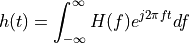
The Fourier Integral is defined by the expression
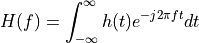
The spectrum  is complex.

with  the real part of the spectrum,
  the imaginary part of the spectrum,
 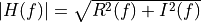 the amplitude of the spectrum,
 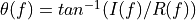 the phase of the spectrum.
The inverse Fourier Integral reconstructs the time-domain signal out of the spectrum.
The collection  is called a Fourier Transform Pair.
Among the many possible Fourier Transform Pairs, one is particularly useful to keep in mind: the Fourier transform of a symmetrical-pulse time-domain waveform. This time-domain signal results in a sinc-shaped frequency spectrum. A bounded time-domain representation thus results in an unbounded frequency-domain representation.
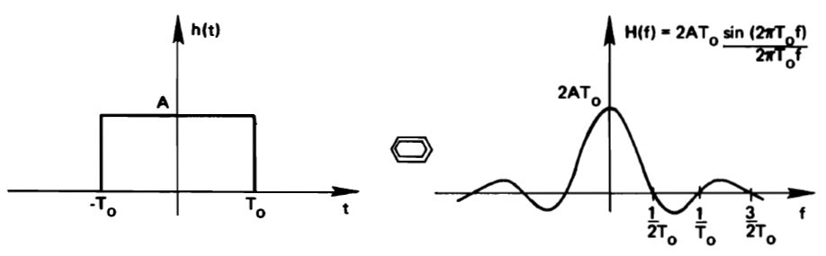
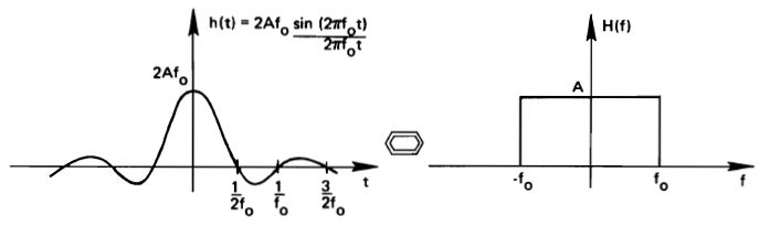
The dual of a symmetrical-pulse time-domain waveform is a pulse-frequency spectrum. In this case, a bounded frequency-domain representation results in an unbounded time-domain signal. Notice the following important characteristic: a time-bounded waveform has an unbounded spectrum, while a frequency-bounded spectrum has an unbounded time-domain representation.
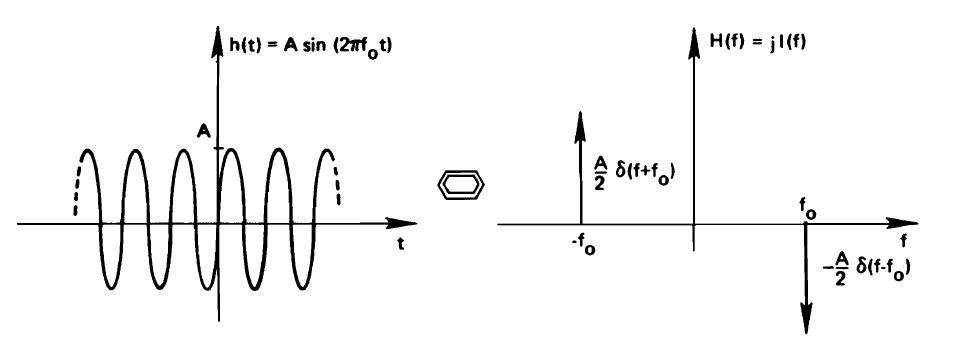
If we analyze periodic functions in time, the spectrum will become discrete and will consist of a collection of Dirac impulses. The periodic nature of the time-domain signal accumulates all the energy at a few locations in the spectrum (at the ground frequency and multiples of the ground frequency, i.e., the harmonics). This results in a spectrum consisting of impulses.
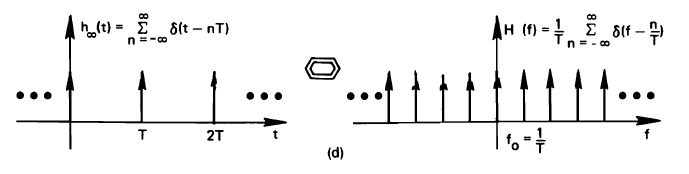
An discrete Fourier Transform pair that is particularly useful to keep in mind is the pulse stream, namely, the spectrum created by a series of time-domain pulses. We discussed this Fourier transform pair at the start of the course, as well, to describe the sampling process.
Convolution and Multiplication
Many time-domain operations have a corresponding frequency-domain operation. But one operation stands out above others for its importance to understand frequency-domain properties. That operation pair is convolution and multiplication.
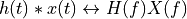
The convolution operation, denoted by the symbol  , is defined as follows.
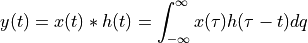
The convolution operation describes the response of a linear system described by an impulse response  on an input signal
  . Convolution in the time-domain is connected to multiplication in the frequency domain (of corresponding signal spectra). Conversely, multiplication in the time-domain is connected to convolution in the frequency domain (of corresponding spectra). Formally, given two Fourier Transform Pairs, and
  , the following properties hold.
and
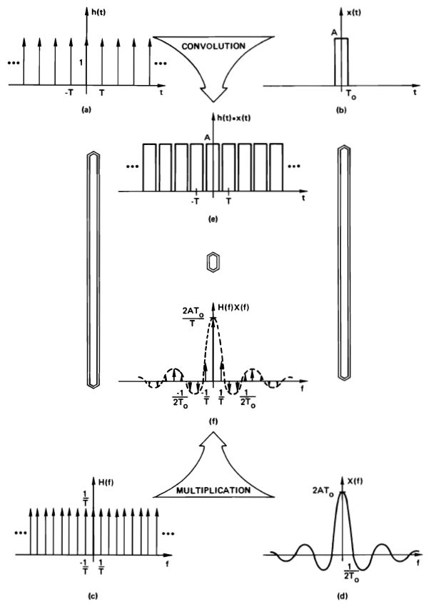
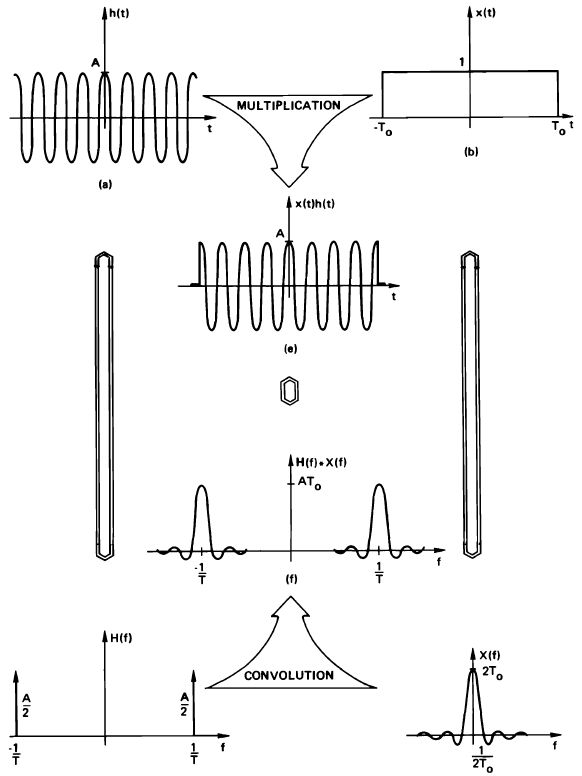
The usefulness of these properties becomes apparent when we derive the spectrum of complex signals. For example, consider how the spectrum of a block-train signal can be computed. The signal is periodic, so we know it must have a discrete spectrum. Realizing that the time-domain signal is the result of convolving a block with a pulse train, we can then derive the spectrum of a block train by multiplying the spectrum of a pulse train and a block.
A similar argument can be made about a bounded (but repetitive) time-domain signal. For example, a cosine is multiplied by a rectangular window to create a complex time-limited signal. For such a signal, we know that the spectrum will be continuous and infinite. Realizing that the spectrum of a cosine is just two pulses, and the spectrum of a rectangular window is a sinc function, we can thus infer that the spectrum of the bounded cosine function will have a sync shape, as well, centered around the cosine frequency.
Development of the Discrete Fourier Transform
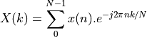
We have now all the tools we need to describe and understand the operation of the DFT. The Discrete Fourier Transform is defined as follows.
The DFT is similar to the Fourier Transform, but not identical to it. Note that the DFT is computed over a limited quantity of N samples. The DFT is period: it describes the spectrum of a periodic sequence of N samples. Both the time-domain representation and the frequency domain representation are discrete: the DFT is used to describe periodic signals, and it will do so using periodic spectra.
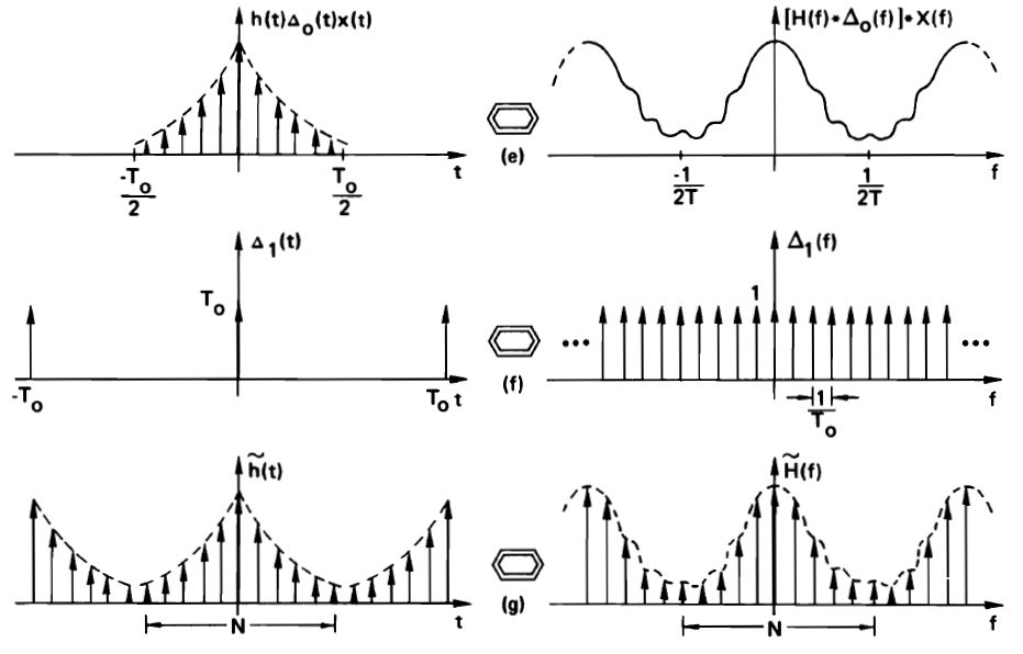
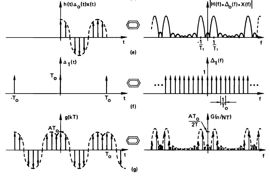
Here is a graphical development of the DFT for a given signal. All of the following are representations of Fourier Transform pairs. First, we need to create a sampled-data representation - in this case of a non-periodic waveform. The sampling operation in the time domain is a multiplication of a pulse train with the continuous, non-period waveform. Some aliasing may unavoidable when the sample frequency is too low.
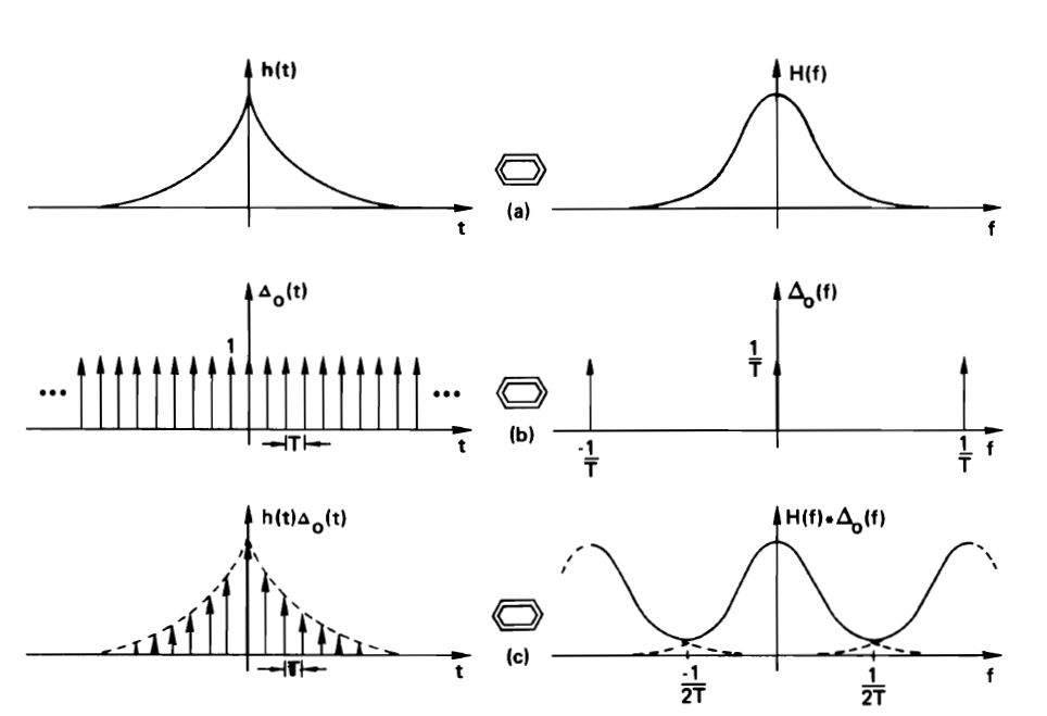
Next, we will bound the time-domain signal in time, to a window of N samples (that will be repated over and over again, when the signal is periodic).
This bounding is implemented by time-windowing the domain-domain pulse stream. In the frequuency domain, we will convolve the periodic continuous spectrum with a sinc spectrum corresponding to the time window. The resulting effect is a ringing in the spectrum. This ringing is caused by the truncation of the time domain signal. The stronger the trunction, the heavier the ringing.
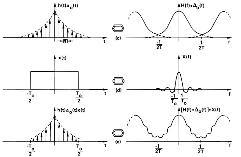
Finally, we make the time-domain representation periodic, so that we get a discrete and periodic time-domain waveform as well as a describe and periodic spectrum. This requires a time-domain convolution with a pulse waveform spectrum, and corresponds to sampling of the spectrum in the frequency domain.
It’s clear that the DFT spectrum is similar to the continuous-time Fourier spectrum, with some caveats.
The time-domain sampling may result in aliasing in the frequency domain. Some of the spectral components in a DFT spectrum may in fact come from an aliased spectrum. The sample frequency of a discrete-time signal must be sufficiently large to minimize aliasing.
To number of samples in a DFT must be sufficiently large to capture every feature of interest.
Effect of Truncation in the Time Domain
When we deal with periodic signals, the DFT must sample the periodic signal over at least one period in order to capture all information. However, we will rarely be able to capture exactly one period. It’s more likely that the sample buffer contains N samples representing a non-integer multiple periods. We will discuss the impact of this sampling over a non-integer multiple of periods.
The resulting distortion is one of the most common issues when working with the DFT or FFT, yet it is generally poorly understood.
First, consider the case where the number of samples N in the DFT captures exactly one period. We have sampled a cosine wave of frequency  at a sample rate of
  . Then, we selected N samples (at sample period
  ) which cover exactly one period. In other words,
  . The resulting spectrum of the truncated cosine wave has a spectrum defined by the convolution of the original signal spectrum with a sinc corresponding to the truncation window. The zeros of the resulting spectrum lie at multiples of .
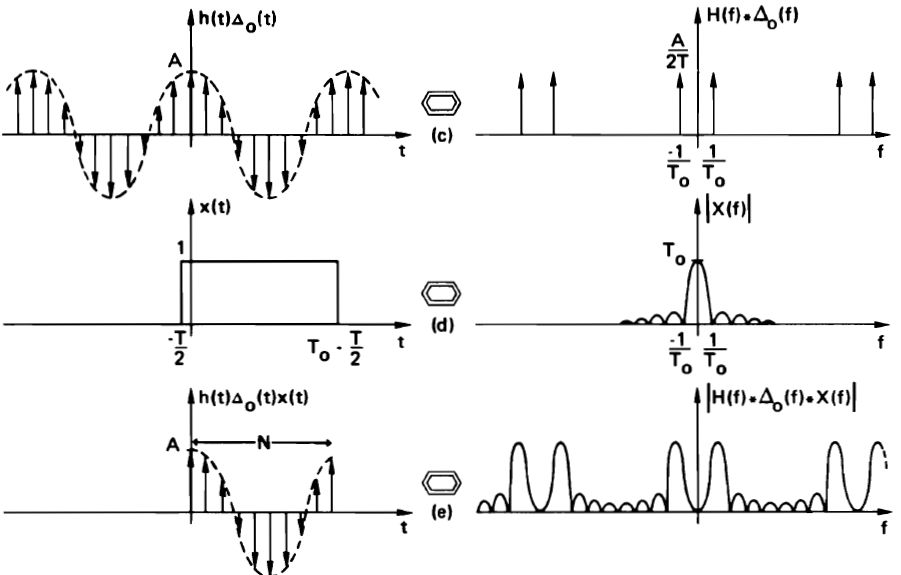
Next, we make the time-domain waveform periodic again, as required for the DFT. This will sample the resulting continuous spectrum into a discrete spectrum. However, the convolution in the time domain
is done with a pulse stream identical to the original period  . In the frequency domain, we sample a continuous sinc spectrum at multiples of . This will ensure that the sampled spectrum contains all the zeros in the continuous spectrum. The discrete spectrum, in this case, is very similar to the original spectrum.
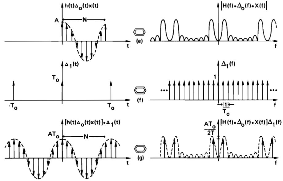
Now, let’s consider what happens when the original sampled waveform is not an integral number of periods.
We now sample a cosine of period  , while we still capture N samples at sample rate so that the truncation window is . From the Figure, we see that is smaller than . In the resulting continuous frequency spectrum, we get a sync shape with zeros at multiples of , with with the main lobe centered around
  .
.
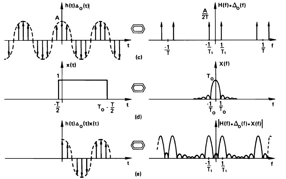
When we make the time waveform periodic again, we will sample the continuous spectrum at .
A serious distortion appears. Because the sinc shape is centered around instead of , we will sample besides the zeros of the sinc, and many non-zero components appear in the spectrum. This distortion is caused by the fact that we have a non-integral number of periods of the signal in our DFT. Therefore, the reconstructed periodic waveform no longer looks like the original periodic waveform. This distortion can be significant.
Understanding the Fast Fourier Transform
The FFT is a faster version of the DFT that introduces a significant reduction on the number
of complex multiplications. The classic DFT requires on the order of  complex
multiplications and about the same number of additions in order to obtain each
frequency sample
complex
multiplications and about the same number of additions in order to obtain each
frequency sample  . The FFT, on the other hand, only requires
  complex multiplications and
  complex additions.
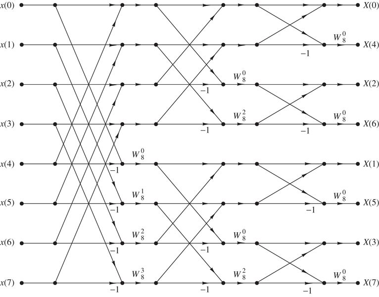
While the detailed derivation of the FFT is beyond this lecture, we will look at the overall structure of the algorithm. Proakis and Manolakis derive the following figure for an 8-point ‘decimation-in-time’ FFT.
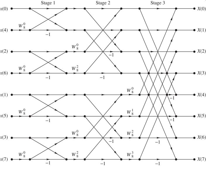
In this figure, ![x[i]](_images/math/77ed45ba10ba1d98a72398b21802def7a79b7717.png) represents time-domain representation, while
represents time-domain representation, while ![X[j]](_images/math/65bdc366106db407363bc32d18ff166a665dfcce.png) represents
frequency-domain representation. The constants
represents
frequency-domain representation. The constants  are twiddle factors and defined by
the expression
are twiddle factors and defined by
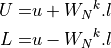
the expression 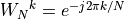 . Hence they represent complex numbers. The algorithm has a great regularity, and is defined by a sequence of butterfly operation, where each butterfly operation transforms two inputs
  into two outputs
  :
:
This is repeated in several stages, which combine inputs that are spaced apart by a power-of-two. The input applies the input signal in a particular order. Rather than processing the input signal as a vector  , the input is applied as
  . This reshuffling is a consequence of the decomposition of the FFT computation in several stages. The data indices are stored in bit-reversed order. Every index of an 8-point FFT can be written in three bits, and the reshuffling required for the decimation-in-time FFT is given by bit-reversing the index. For example, index 3 is
  in binary, and becomes
  in bit-reversed from, or 6. Thus, the element at index 3 has to be inserted at index 6 (and conversely, the element at index 6 has to be inserted at index 3).
An alternate decomposition of the DFT, called ‘decimation-in-frequency’ FFT, starts from an in-order time index and produces frequency samples which are bitreversed. It has the same efficiency gain as the decimation-in-time algorithm.
Resolution of the FFT
The FFT is a very important computational kernel for signal processing
applications. A major application for FFT is, of course, in the computation
of FFT transforms. We have to keep in mind that the FFT computes the DFT and
not the Fourier integral itself. The number of samples, as well as the sample
frequency, are of great importance to have a good approximation of the
Fourier integral. The resolution of the FFT with  points and at
sample rate is defined as
points and at
sample rate is defined as  . The resolution reflects
to the frequency resolution expressed in the FFT, namely, the smallest frequency
difference that can be reflect in the output. Note that, the provide
a higher resolution (that is, a lower value for ), we would
increase rather than , since an increase of
may result in aliasing.
. The resolution reflects
to the frequency resolution expressed in the FFT, namely, the smallest frequency
difference that can be reflect in the output. Note that, the provide
a higher resolution (that is, a lower value for ), we would
increase rather than , since an increase of
may result in aliasing.
If you increase to increase the resolution of the FFT, then you
have to make sure to add additional samples from the input. Merely appending
zeroes, or repeating the input periodically, will not improve the
approximation of the Fourier Transform by the FFT.
Removing the effect of truncation
When the signal converted by the FFT has a non-integral number of periods, then the resulting (FFT-)periodic signal is no longer continuous but has sharp transitions between sample N-1 from a previous (FFT-)period and sample 0 of the current (FFT-)period. Since these sharp transitions do not exist in the original sampled input signal, the resulting FFT will contain frequency components that do not exist in the Fourier Transform of the input signal.
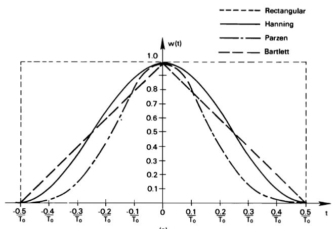
To remove the effect of these transitions, we can reduce the effect of the edges by preprocessing the input signal with a window. For course, the window will affect the frequency content of the input signal. If the number of samples N is large enough, then the impact of windowing is reduced. One of the more popular windowing functions is the Hanning (or Han) window, which is defined by the shape of a cosine function.
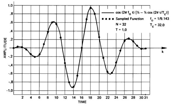
The spectral effect of windowing is that the FFT looses its capability to sharply resolve a given frequency. There is a ‘smearing’ effect, as illustrated by the following figure. A cosine function is sampled in 32 samples. The cosine function includes around 4 periods in 32 samples, but the exact frequency is certainly not one that can be precisely captured with 32 samples. To reduce the ringing effect, the cosine function is windowed with a Hanning windows.
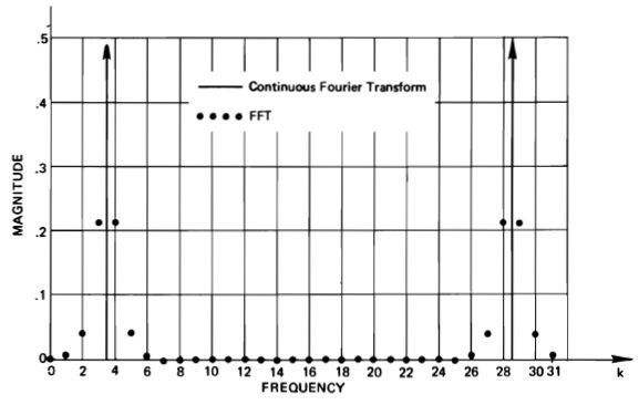
The Fourier transform for this cosine would show two sharp impulses. However, because of
the limited resolution of the FFT (), and because of the smearing effect
produced by the Hanning window, we obtain the following FFT result. Note that this is still
much better than the result that would be obtained using a rectangular window.
The FFT of real input sequences
When the FFT is computed over real input data, half of the input of a complex-valued FFT is unused. Furthermore, the spectrum of such a function shows symmetry: the real part is even, while the imaginary part is odd. This property can be used to compute the FFT of N points of real data using an N/2 point FFT.
First, for a Fourier transform pair 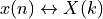 , when
  is real, then
  is an even function and
  is an odd function.
Furthermore, when is imaginary, then is an odd function and is an even function.
is an odd function.
Furthermore, when is imaginary, then is an odd function and is an even function.
Now, the discrete function consisting of N points can be separated in even and odd parts as follows.
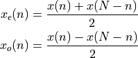
These properties can be used to extract the part of a spectrum belonging to a purely real input, and that belonging to a purely imaginary input. Assume two real signals  and
and  that together form the complex signal
 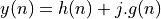 .
.
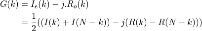
If we compute the frequency response 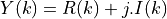 , then the spectrum of and can be expressed in terms of the odd and even parts of
  and
and  . We write the odd and even parts as
  and
and  respectively. The spectra
  and
and  are given by the following expressions.
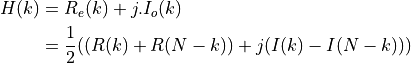
and
Thus, we can use an N-point complex FFT to compute the spetra of two N-point real signals at the same time.
Examples
We next discuss a few examples, provided in the repository for this lecture.
Computation of the DFT
Note
This code for this example is found in the project dft_l11_dft.
A DFT, in general, is computed over a complex input, and will create a complex output. The following program demonstrates a straightforward computation of the DFT using floating point precision.
typedef struct {
  float32_t real;
  float32_t imag;
} COMPLEX;

COMPLEX samples[N];

void dft() {
  COMPLEX result[N];
  int k,n;

  for (k=0 ; k<N ; k++)  {

    result[k].real = 0.0;
    result[k].imag = 0.0;

    for (n=0 ; n<N ; n++) {
      result[k].real += samples[n].real*cosf(2*PI*k*n/N)
                      + samples[n].imag*sinf(2*PI*k*n/N);
      result[k].imag += samples[n].imag*cosf(2*PI*k*n/N)
                      - samples[n].real*sinf(2*PI*k*n/N);
    }
  }

  for (k=0 ; k<N ; k++) {
    samples[k] = result[k];
  }
}
This code is extremely slow, because it computes sine and cosine in real time. A straightforward optimization is to pre-compute the twiddle factors (cosine and sine functions) and store these in an array. We then get the following design.
Note
This code for this example is found in the project dft_l11_dft_twiddle.
typedef struct {
  float32_t real;
  float32_t imag;
} COMPLEX;

COMPLEX samples[N];
COMPLEX twiddle[N];

void inittwiddle() {
    int i;
    for(i=0 ; i<N ; i++) {
        twiddle[i].real =  cos(2*M_PI*i/N);
        twiddle[i].imag = -sin(2*M_PI*i/N);
    }
}

void dft() {
  COMPLEX result[N];
  int k,n;

  for (k=0 ; k<N ; k++)  {

    result[k].real = 0.0;
    result[k].imag = 0.0;

    for (n=0 ; n<N ; n++) {
         result[k].real += samples[n].real*twiddle[(n*k)%N].real
                         - samples[n].imag*twiddle[(n*k)%N].imag;
         result[k].imag += samples[n].imag*twiddle[(n*k)%N].real
                         + samples[n].real*twiddle[(n*k)%N].imag;
    }
  }

  for (k=0 ; k<N ; k++) {
    samples[k] = result[k];
  }
}
This is about three times faster, but it still has quadratic complexity.
Computation of the FFT
The following implementation uses an FFT kernel provided through the ARM CMSIS
library. It uses 64 points of complex data. Rather than using a COMPLEX record,
it uses a floating-point array of 2*64 entries. This code shows not only the actual
call to the library, but also the integration in a function that is compatible with
the DMA-based method in the BOOSTXL library. Hence, the DMA will collect 64 samples,
feed them into the FFT buffer, compute the DFT, and next extract the real data to
the output (note that we are ignoring the imaginary part of the output). The idea
of this program is that it can display the spectrum on an oscilloscope in real time.
Note
This code for this example is found in the project dft_l11_fft_cmsis.
float32_t samples[2*N];

void perfCheck(uint16_t x[BUFLEN_SZ], uint16_t y[BUFLEN_SZ]) {
    int i;
    for (i=0; i<N; i=i+1) {
        samples[2*i]     = adc14_to_f32(x[i]);
        samples[2*i + 1] = 0.0;
    }
    arm_cfft_f32(&arm_cfft_sR_f32_len64, samples, 0, 1);
    for (i=0; i<N; i=i+1) {
        y[i] = f32_to_dac14(0.1*(samples[2*i]*samples[2*i] +
                                 samples[2*i+1]*samples[2*i+1]));
    }
}
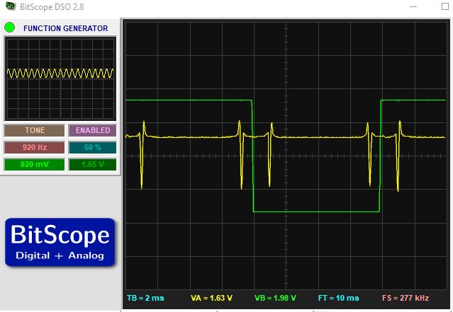
This program is 30 times faster than the original DFT, clearly justifying the FFT algorithm. The monitor the spectrum, we inject a tone (sinus) in the input pin and observe the output. The duty cycle pin level (in green) marks the phase of the DMA I/O cycle, thereby separating multiple spectra. Thus is the response to a 920Hz input signal.
The program can be optimized further by using a library call that is optimized for real data. Such a call can use an N/2 point complex FFT to compute an N point real FFT.
Note
This code for this example is found in the project dft_l11_fft_cmsis_real.
arm_rfft_fast_instance_f32 armFFT;

void initfft() {
    arm_rfft_fast_init_f32(&armFFT, N);
}

void perfCheck(uint16_t x[BUFLEN_SZ], uint16_t y[BUFLEN_SZ]) {
    int i;

    for (i=0; i<N; i++)
        insamples[i] = adc14_to_f32(x[i]);

    arm_rfft_fast_f32(&armFFT, insamples, outsamples, 0);

    for (i=0; i<N; i = i + 2)
        y[i] = y[i+1] = f32_to_dac14(0.1*(outsamples[i]*outsamples[i] +
                                          outsamples[i+1]*outsamples[i+1]));

}
This program still runs 25% faster then the complex FFT. However, it exhibits severe distortion because of truncation effects, as discussed earlier. To solve this, we will apply a windowing over the input, which gradually tapers of the influence of points at the boundary of the window towards zero. Once such a window is called a Han function (aka Hanning Window or Raised Cosine Window).
Note
This code for this example is found in the project dft_l11_fft_cmsis_real_hanning.
arm_rfft_fast_instance_f32 armFFT;

void initsamples() {
    int i;
    for(i=0 ; i<N ; i++)
        insamples[i] = 0.01 * cosf(2*M_PI*TESTFREQ*i/SAMPLING_FREQ);
}

void initfft() {
    int i;
    for(i=0 ; i<N ; i++)
        hanning[i] = sinf(M_PI*i/N) * sinf(M_PI*i/N);
    arm_rfft_fast_init_f32(&armFFT, N);
}

void perfCheck(uint16_t x[BUFLEN_SZ], uint16_t y[BUFLEN_SZ]) {
    int i;

    for (i=0; i<N; i++)
        insamples[i] = adc14_to_f32(x[i]) * hanning[i];

    arm_rfft_fast_f32(&armFFT, insamples, outsamples, 0);

    for (i=0; i<N; i++)
        y[i] = f32_to_dac14(outsamples[i]);

}
Here is a summary of the resulting cycle counts.
Code |
Cycle Count |
Remarks |
|---|---|---|
dsp_l11_dft |
3906787 |
Complex DFT, N = 64 |
dsp_l11_dft_twiddle |
966584 |
Complex DFT, precomputed W, N=64 |
dsp_l11_fft_cmsis |
37131 |
Complex FFT, N = 64 |
dsp_l11_fft_cmsis_real |
28430 |
Real FFT, N = 64 |
dsp_l11_fft_cmsis_real_hanning |
29401 |
Real FFT, N = 64, Hanning |
Conclusions
This lecture has covered quite some ground in the computation of the spectrum of a signal. We analyzed the computation of the Discrete Fourier Transform and its relationship to the Fourier Integral in detail. We discussed effects such as truncation of the signal in the time domain. The FFT is an algorithm that enables fast computation of the DFT, and it is the mainstream solution to compute the spectrum on digital computers. Several examples, some of which were based on the ARM CMSIS library, demonstrated the the FFT is much faster than the DFT.