The Fast Fourier Transform
The purpose of this lecture is as follows.
To describe relationship between Fourier Transform, Fourier Series, Discrete Time Fourier Transform, and Discrete Fourier Transform
To describe a fast implementation of the DFT called the Fast Fourier Transform
To demonstrate several implementations in C of the FFT
To describe and demonstrate parctical aspects of implementation of the DFT and FFT
Attention
The examples for this lecture are available as https://github.com/wpi-ece4703-b24/fourier
The Fourier Transform for Periodic and Discrete Signals
There are four major forms of Fourier Transforms, which are based on whether we are dealing with discrete or continuous functions, and whether we are dealing with periodic or non-period functions.
First, there are four different transforms. They all boil down, in essence, to the Fourier Integral. However, the nature of the signals requires special techniques to be used to compute the Fourier Integral - and this gives rise to different Fourier Transform computation techniques.
Non-periodic Signal |
Periodic Signal |
|
Continuous Time |
Fourier Transform |
Fourier Series |
Discrete Time |
Discrete Time Fourier Transform |
Discrete Fourier Transform |
Second, the spectrum computed by each of these four transforms is different. The nature of the time-domain signal (discrete or continuous, and periodic or not), is reflected in the nature of the spectrum.
Time Domain |
Non-periodic Signal |
Periodic Signal |
Continuous Time |
Continuous Non-periodic Spectrum |
Discrete Non-periodic Spectrum |
Discrete Time |
Continuous Periodic Spectrum |
Discrete Periodic Spectrum |
These four cases all describe the same activity: they convert a time-domain representation into a frequency-domain representation and vice-versa.
The real world is always analog and continuous. And very often, physical phenomena are timelimited and not truly periodic in a mathematical sense. Yet, Digital Signal Processing (which runs on digital computers) works by definition always with discrete-time signals and discrete-frequency signals. The mere act of analog to digital conversion removes the continuous character of a time-domain signal. Furthermore, DSP programs describe, by definition, a periodic process.
DSP programs transform an infinite stream of samples, applying the same type of processing to each sample. The spectral analysis tool implemented by a DSP program is a DFT - even if we’re interested in actually computing a Fourier Transform or a Fourier Series. Therefore, we have to build insight on the intepretation of the DFT results.
In this lecture, we’ll look at a particular implementation of the DFT Transform. We will treat the FFT algorithm as a given and will not derive it. However, we will investigate why it is called the Fast Fourier Transform.
Attention
Many of the figures in these lectures notes are taken from the excellent treatment of FFT by E.O. Brigham (The Fast Fourier Transform and its Applications, Prentice Hall, 1988). It’s out of print but it’s relatively easy to find a second-hand copy.
Understanding the Discrete Fourier Transform
In this first section, we will systematically build insight into the DFT and its properties.
The Fourier Transform and Properties
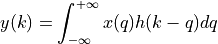
The Fourier Integral is defined by the expression
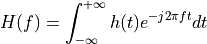
The spectrum  is complex.

with  the real part of the spectrum, and
  the imaginary part of the spectrum.
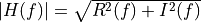 is the amplitude of the spectrum, and
 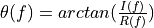 is the phase of the spectrum.
The inverse Fourier Integral reconstructs the time-domain signal from the spectrum.
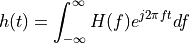
The Fourier Transform pair is the combination  .
.
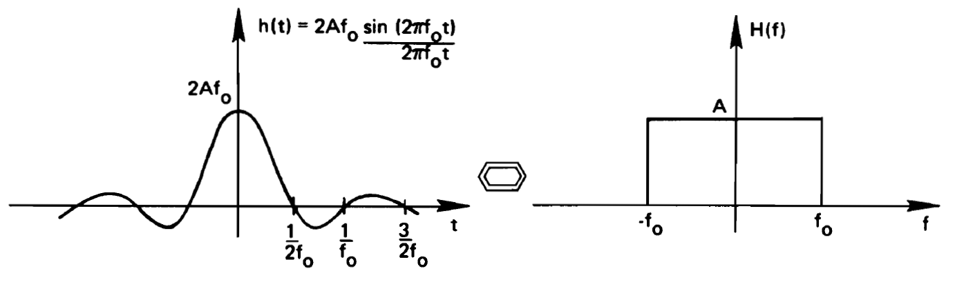
Among the many possible Fourier Transform Pairs, one is particularly useful to keep in mind: the Fourier transform of a symmetrical-pulse time-domain waveform.
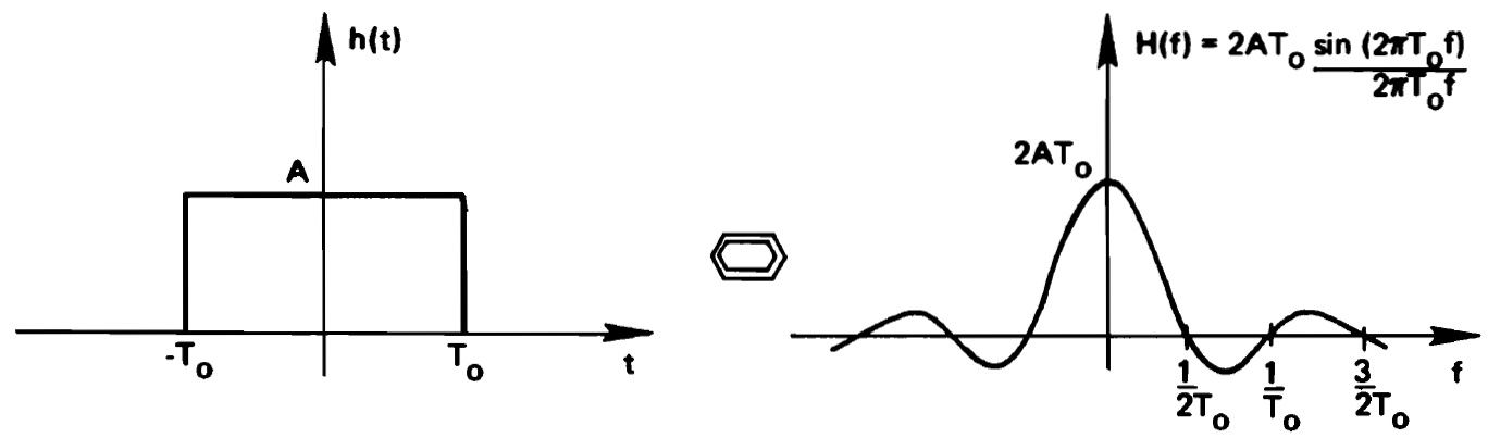
The dual of a symmetrical-pulse time-domain waveform is a sinc-frequency waveform. Notice the following important characteristic: a time-bounded waveform has an unbounded spectrum, while a frequency-bounded spectrum has an unbounded time-domain representation.
If we analyze periodic functions in time, the spectrum will become discrete and will consist of a collection of Dirac impulses. The periodic nature of the time-domain signal accumulates all the energy at a few locations in the spectrum (at the ground frequency and multiples of the ground frequency, i.e., the harmonics).
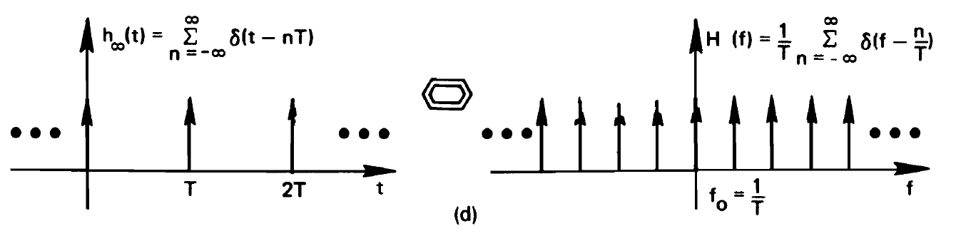
Another Fourier Transform pair that is particularly useful to keep in mind is the pulse stream, namely, the spectrum created by a series of time-domain pulses. We discussed this Fourier transform pair at the start of the course, as well, to describe the sampling process.
Convolution and Multiplication
Many time-domain operations have a corresponding frequency-domain operation. But one operation stands out above others for its importance to understand frequency-domain properties. That operation pair is convolution and multiplication.
The convolution operation, denoted by the symbol  , is defined as follows.
The convolution operation describes the response of a linear system described by an impulse response  on an input signal
  . Convolution in the time-domain is connected to multiplication in the frequency domain (of corresponding signal spectra). Conversely, multiplication in the time-domain is connected to convolution in the frequency domain (of corresponding spectra). Formally, given two Fourier Transform Pairs,
  and
and  , the following properties hold.
and
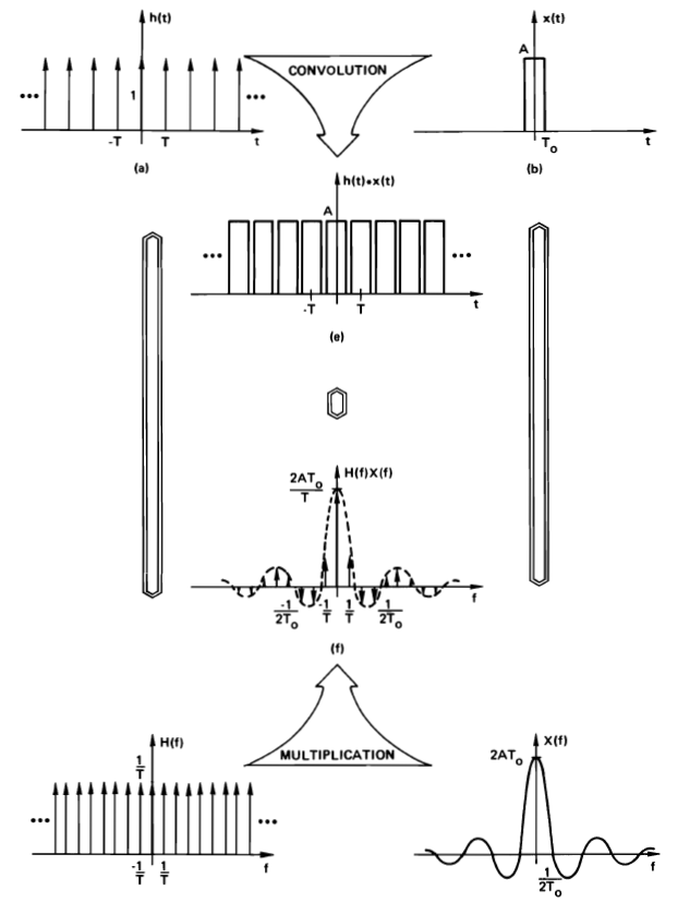
The usefulness of these properties becomes apparent when we derive the spectrum of composite signals, i.e. signals that can be expressed as a composition of simple signals. For example, consider how the spectrum of a block-train signal can be computed. The signal is periodic, so we know it must have a discrete spectrum. The spectrum of a block train can be derived from the spectrum of a pulse train and the spectrum of a block.
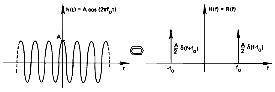
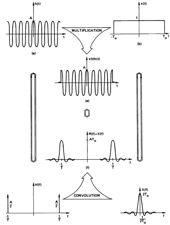
A similar argument can be made about a bounded (but repetitive) time-domain signal. For example, a cosine is multiplied by a rectangular window to create a complex time-limited signal. For example, a cosine is multiplied by a rectangular window to create a complex time-limited signal.
For such a signal, we know that the spectrum will be continuous and infinite. Realizing that the spectrum of a cosine is just two pulses, and the spectrum of a rectangular window is a sinc function, we can thus infer that the spectrum of the bounded cosine function will have a sinc shape, as well, centered around the cosine frequency.
Development of the Discrete Fourier Transform
We have now all the tools we need to describe and understand the operation of the DFT. The Discrete Fourier Transform is defined as follows.
The DFT is similar to the Fourier Transform, but not identical to it. Note that the DFT is computed over a limited quantity of N samples. Also, both the time-domain representation and the frequency domain representation are discrete: the DFT is used to describe periodic signals, and it will do so using periodic spectra.
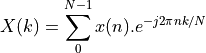
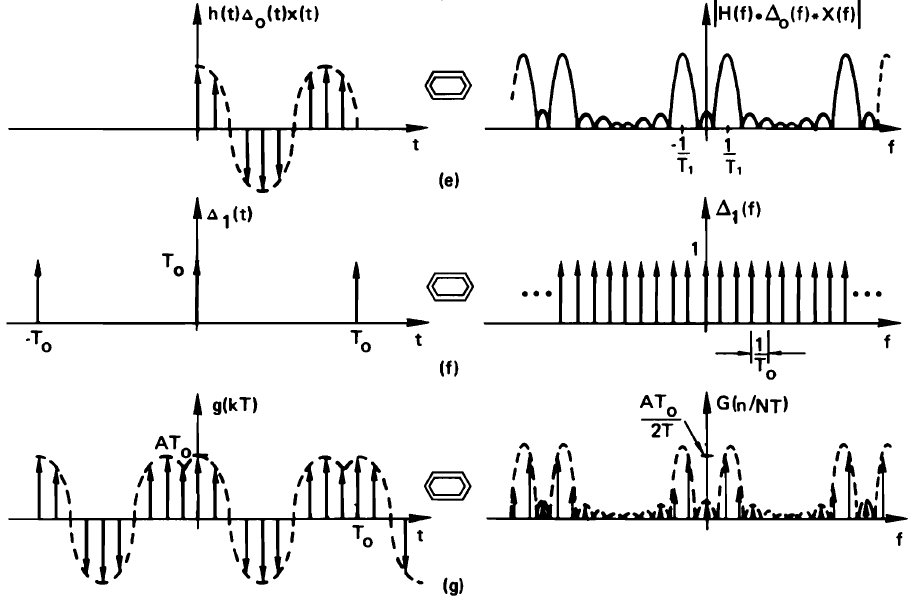
Here is a graphical development of the DFT for a given signal. All of the following are representations of Fourier Transform pairs. First, we need to create a sampled-data representation - in this case of a non-periodic waveform. The sampling operation in the time domain is expressed a multiplication with a pulse train. Some aliasing may unavoidable in case the sample frequency is too low
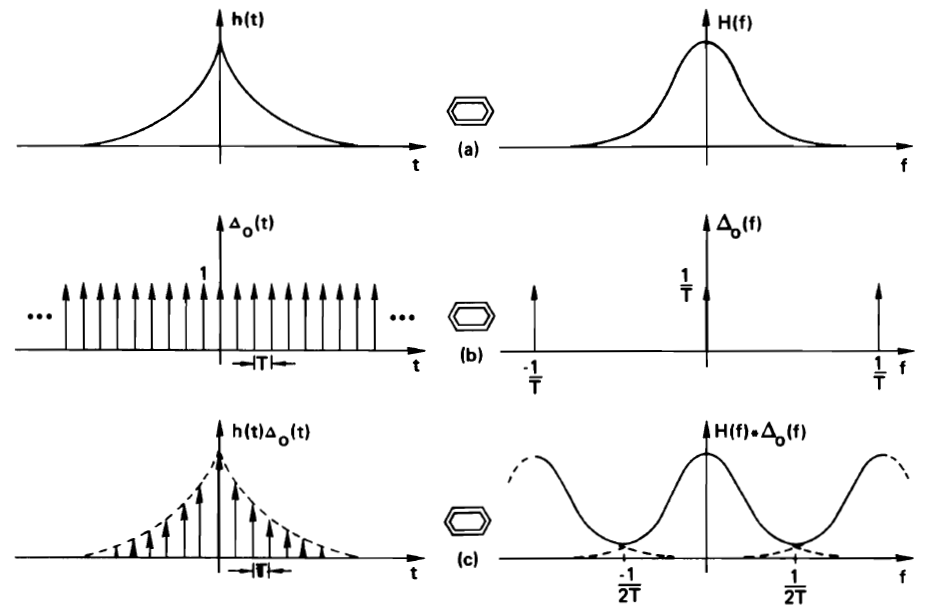
Next, we will bound the time-domain signal in time, to a window of N samples. This is implemented by time-windowing the domain-domain pulse stream. In the frequency domain, we will convolve the periodic continuous spectrum with a sinc spectrum corresponding to the time window. The resulting effect is a ringing in the spectrum. This ringing is caused by the truncation of the time domain signal. The stronger the truncation, the heavier the ringing.
Finally, we make the time-domain representation periodic, so that we get a discrete and periodic time-domain waveform as well as a periodic spectrum. This requires a time-domain convolution with a pulse waveform spectrum, and corresponds to sampling of the spectrum in the frequency domain.
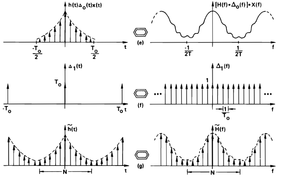
It’s clear that the DFT spectrum is similar to the continuous-time Fourier spectrum, with some caveats.
The time-domain sampling may result in aliasing in the frequency domain. Some of the spectral components in a DFT spectrum may in fact come from an aliased spectrum. The sample frequency of a discrete-time signal must be sufficiently large to minimize aliasing.
The frequency-domain sampling may result in truncation of important features in the time domain. To number of samples in a DFT must be sufficiently large to capture every feature of interest.
Effect of Truncation in the Time Domain
When we deal with periodic signals, the DFT must sample the periodic signal over at least one period in order to capture all information. However, we will rarely be able to capture exactly one period. It’s more likely that the sample buffer contains N samples representing a non-integer multiple periods. We will discuss the impact of this sampling over a non-integer multiple of periods.
The resulting distortion is one of the most common issues when working with the DFT or FFT, yet it is generally poorly understood.
First, consider the case where the number of samples N in the DFT captures exactly one period. We have sampled a cosine wave of frequency  at a sample rate of
  . Then, we selected N samples (at sample period T) which cover exactly one period. In other words,
  . The resulting spectrum of the truncated cosine wave has a spectrum defined by the convolution of the original signal spectrum with a a sinc corresponding to the truncation window. The zeros of the resulting spectrum lie at multiples of .
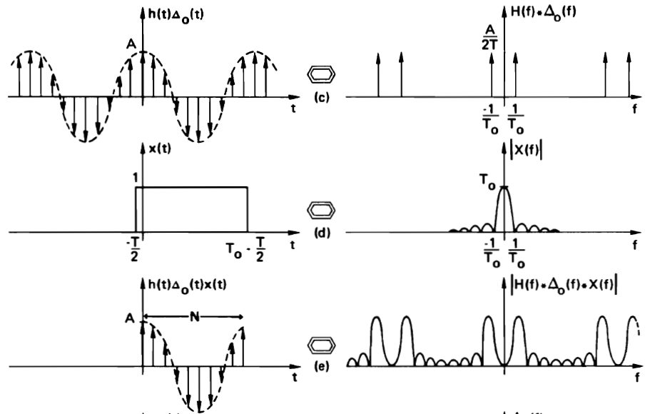
Next, we make the time-domain waveform periodic again, as required for the DFT. This will sample the resulting continuous spectrum into a discrete spectrum. However, the convolution in the time domain is done with a pulse stream identical to the original period. In the frequency domain, where we sample a continuous sinc spectrum at multiples of . This will ensure that the sampled spectrum contains all the zeros in the continuous spectrum. The discrete spectrum, in this case, is very similar to the original spectrum.
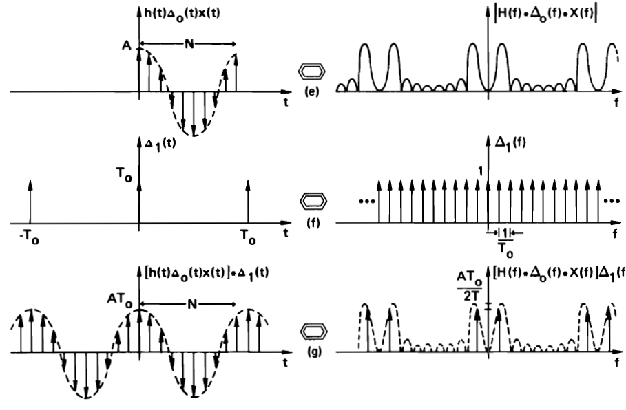
Now, let’s consider what happens when the original sampled waveform is not an integral number of periods. We now sample a cosine of period  , while we still capture N samples at sample rate so that the truncation window is . From the Figure, we see that is smaller than
  . In the resulting continuous frequency spectrum, we get a sync shape with zeros at lobe centered around
  .
.
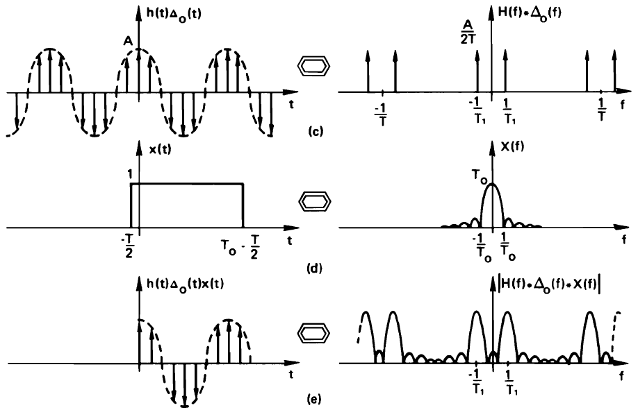
When we make the time waveform periodic again, we will sample the continuous spectrum at . And now, a serious distortion happens. Because the sinc shape is centered around instead of , we will sample besides the zeros of the sinc, and many non-zero components appear in the spectrum. This distortion is caused by the fact that we have a non-integral number of periods of the signal in our DFT. Therefore, the reconstructed periodic waveform no longer looks like the original periodic waveform. This distortion can be significant, and we will discuss a method to minimize it when we go over programming examples.
The Fast Fourier Transform
The core idea of the Fast Fourier Transform, due to Cooley and Tukey, is to decompose the DFT, shown above, in multiple passes to exploit the symmetry of multiplying with  , which is periodic. A detailed elaboration of the algorithm is out of scope of this lecture, and we merely capture the gist of it. However, it is probably the most important algorithms in signal processing because its widespread use. Indeed, while the direct DFT has quadratic complexity, the FFT has complexity
  , with
  the number of points in the FFT transformation. Without it, many real-time operations in signal processing would be impossible.
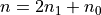
Considering the DFT anove, and decomposing  and
and  in individual bits, we can write a 4-point DFT as follows.
where 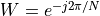 ,
,  and
and  . Next, we rewrite the
  term to bring out symmetry.
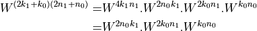
The term  is always 1.
We thus rewrite the DFT as follows.
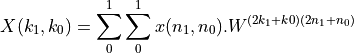
![X(k_1, k_0) = \sum_{n_0=0}^{1} \left[ \sum_{n_1=0}^{1} x(n_1,n_0).W^{2k_0n_1} \right] W^{(2k_1 + k0)n_0}](_images/math/4910a113610888eaae53720930ea63bc2607bd6e.png)
The FFT is developed by computing the inner sum followed by the outer sum. Thus, we first compute
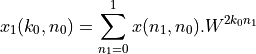
which leads to the following set of intermediate results:
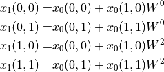
Once we have  , we compute the outer sum as follows.
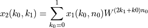
which leads to the following set of results:
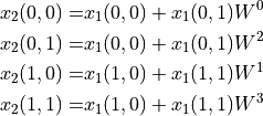
Finally, we have obtained 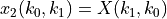 . In other words. the order of the results
in
. In other words. the order of the results
in  are in bit-reversed index order.
Graphically, we summarize these operations as follows.
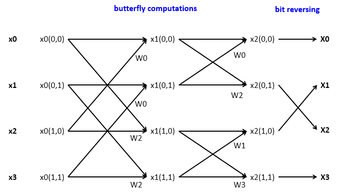
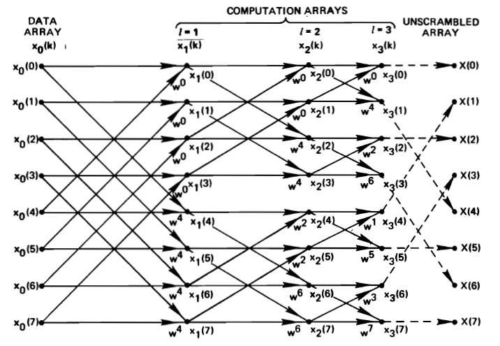
This expands to higher powers of two as well. We have  stages of butterfly computations, followed
by a bit-reversing of the output result. For example, this is the flow diagram for an 8-point FFT.
stages of butterfly computations, followed
by a bit-reversing of the output result. For example, this is the flow diagram for an 8-point FFT.
Examples
We next discuss a few examples, refer to the repository for this lecture.
Computation of the DFT
A DFT, in general, is computed over a complex input, and will create a complex output. The following program demonstrates a straightforward computation of the DFT using floating point precision.
typedef struct {
  float32_t real;
  float32_t imag;
} COMPLEX;

COMPLEX samples[N];

#define TESTFREQ 3000.0
#define SAMPLING_FREQ 8000.0

void initsamples() {
    int i;
    for(i=0 ; i<N ; i++) {
        samples[i].real = 0.01 * cosf(2*M_PI*TESTFREQ*i/SAMPLING_FREQ);
        samples[i].imag = 0.0;
    }
}

void dft() {
  COMPLEX result[N];
  int k,n;

  for (k=0 ; k<N ; k++)  {

    result[k].real = 0.0;
    result[k].imag = 0.0;

    for (n=0 ; n<N ; n++) {
      result[k].real += samples[n].real*cosf(2*PI*k*n/N)
                      + samples[n].imag*sinf(2*PI*k*n/N);
      result[k].imag += samples[n].imag*cosf(2*PI*k*n/N)
                      - samples[n].real*sinf(2*PI*k*n/N);
    }
  }

  for (k=0 ; k<N ; k++) {
    samples[k] = result[k];
  }
}
This code is extremely slow, because it computes sine and cosine in real time. A straightforward optimization is to pre-compute the twiddle factors (cosine and sine functions) and store these in an array. We then get the following design.
typedef struct {
  float32_t real;
  float32_t imag;
} COMPLEX;

COMPLEX samples[N];
COMPLEX twiddle[N];

void inittwiddle() {
    int i;
    for(i=0 ; i<N ; i++) {
        twiddle[i].real =  cos(2*M_PI*i/N);
        twiddle[i].imag = -sin(2*M_PI*i/N);
    }
}

void dft() {
  COMPLEX result[N];
  int k,n;

  for (k=0 ; k<N ; k++)  {

    result[k].real = 0.0;
    result[k].imag = 0.0;

    for (n=0 ; n<N ; n++) {
         result[k].real += samples[n].real*twiddle[(n*k)%N].real
                         - samples[n].imag*twiddle[(n*k)%N].imag;
         result[k].imag += samples[n].imag*twiddle[(n*k)%N].real
                         + samples[n].real*twiddle[(n*k)%N].imag;
    }
  }

  for (k=0 ; k<N ; k++) {
    samples[k] = result[k];
  }
}
This is about three times faster, but it still has quadratic complexity.
Computation of the FFT
The following implementation uses an FFT kernel provided through the ARM CMSIS library. It uses 64 points of complex data. Rather than using a COMPLEX record, it uses a floating-point array of 2*64 entries. This code shows not only the actual call to the library, but also the integration in a function that is compatible with the DMA-based method in the XLAUDIO_LIB. Hence, the DMA will collect 64 samples, feed them into the FFT buffer, compute the DFT, and next extract the real data to the output (note that we are ignoring the imaginary part of the output). The idea of this program is that it can display the spectrum on an oscilloscope in real time.
float32_t samples[2*N];

void perfCheck(uint16_t x[BUFLEN_SZ], uint16_t y[BUFLEN_SZ]) {
    int i;
    for (i=0; i<N; i=i+1) {
        samples[2*i]     = adc14_to_f32(x[i]);
        samples[2*i + 1] = 0.0;
    }
    arm_cfft_f32(&arm_cfft_sR_f32_len64, samples, 0, 1);
    for (i=0; i<N; i=i+1) {
        y[i] = f32_to_dac14(0.1*(samples[2*i]*samples[2*i] +
                                 samples[2*i+1]*samples[2*i+1]));
    }
}
This program is 30 times faster than the original DFT, clearly justifying the FFT algorithm. The program can be optimized further by using a library call that is optimized for real data. Such a call can use an N/2 point complex FFT to compute an N point real FFT.
arm_rfft_fast_instance_f32 armFFT;

void initfft() {
    arm_rfft_fast_init_f32(&armFFT, N);
}

void perfCheck(uint16_t x[BUFLEN_SZ], uint16_t y[BUFLEN_SZ]) {
    int i;

    for (i=0; i<N; i++)
        insamples[i] = adc14_to_f32(x[i]);

    arm_rfft_fast_f32(&armFFT, insamples, outsamples, 0);

    for (i=0; i<N; i = i + 2)
        y[i] = y[i+1] = f32_to_dac14(0.1*(outsamples[i]*outsamples[i] +
                                 outsamples[i+1]*outsamples[i+1]));

}
This program still runs 25% faster then the complex FFT. However, it exhibits severe distortion because of truncation effects, as discussed earlier. To solve this, we will apply a windowing over the input, which gradually tapers of the influence of points at the boundary of the window towards zero. Once such a window is called a Hanning function (aka Hanning Window or Raised Cosine Window).
arm_rfft_fast_instance_f32 armFFT;

void initsamples() {
    int i;
    for(i=0 ; i<N ; i++)
        insamples[i] = 0.01 * cosf(2*M_PI*TESTFREQ*i/SAMPLING_FREQ);
}

void initfft() {
    int i;
    for(i=0 ; i<N ; i++)
        hanning[i] = sinf(M_PI*i/N) * sinf(M_PI*i/N);
    arm_rfft_fast_init_f32(&armFFT, N);
}

void perfCheck(uint16_t x[BUFLEN_SZ], uint16_t y[BUFLEN_SZ]) {
    int i;

    for (i=0; i<N; i++)
        insamples[i] = adc14_to_f32(x[i]) * hanning[i];

    arm_rfft_fast_f32(&armFFT, insamples, outsamples, 0);

    for (i=0; i<N; i = i+2)
        y[i] = y[i+1] = f32_to_dac14(outsamples[i] * outsamples[i] + outsamples[i+1] * outsamples[i+1]);

}
Performance Summary
We thus end with the following performance results.
Code |
Cycle Count |
Remarks |
|
3,000,247 |
Complex DFT, N=64 |
|
199,349 |
Complex DFT, precomputed W, N=64 |
|
34,255 |
Complex FFT, N=64 |
|
24,119 |
Real FFT, N=64 |
|
24,710 |
Real FFT, N=64, Hanning |