Lecture 15 - Synchronous Dataflow
- Introduction
- Basics of Dataflow Modeling
- Multi-input Multi-output Actors
- Multi-rate Actors and Multi-rate Dataflow
- Analysis of multi-rate Dataflow systems
- Applications and Limitations of Dataflow
- Further reading on dataflow
Introduction
In this lecture we will take a step back from the low-level details of custom instructions and the conversion of C code to Verilog code. Instead, we consider the problem of how to capture functionality at a high level of abstraction. In this context, a high level of abstraction means a behavioral level with no distinction between hardware and software.
Such a high-level modeling is popular for many different kinds of engineering problems. Think of Matlab and all its toolboxes to target different problem domains, for example. In the area of computer engineering, high level modeling is used to build an initial understanding of the requirements of a specification, while leaving out most of the detailed design decisions.
For example, a high-level model may express the functionality of an implementation, without addressing the detailed timing or performance characteristics. A high-level model may express how different submodels of a complete design communicate with each other, without providing a detailed implementation for each of the submodels.
The high-level modeling mechanism that we will discuss today is called synchronous data-flow. Synchronous data-flow is a model of computation, a high-level model that comes with precise rules of execution. You’re already familiar with one other very popular model of computation called Finite State Machines. Synchronous Dataflow is a modeling technique similar to FSM, but unlike FSM it is focused on describing computations rather than control state transitions.
Synchronous Dataflow provides the following advantages.
-
Dataflow models are uncommitted: they can express hardware behavior, software behavior, or both. Of course, uncommitted does not mean that a dataflow model can replace C and Verilog. It only means that dataflow models enable you to capture system behavior before you have to think about detailed C code or Verilog code.
-
Dataflow models are concurrent. Dataflow models can express sequential systems as well as parallel systems (where multiple activities happen simultaneously). It’s precisely this feature that makes them so useful for hardware-software codesign. Dataflow models can express the parallelism between hardware and software.
In addition to these advantages, synchronous dataflow models have limitations. We will elaborate on these disadvantages further down.
Basics of Dataflow Modeling
A dataflow model abstracts system behavior as a graph. The nodes in the graph represent subfunctions of the system. The edges in the graph represent communication links. These edges connect the nodes in the graph, and they establish data dependencies between the subfunctions.
Consider the following system with three edges and two nodes, A and B.
This is a system with a first subfunction A and a second subfunction B. A receives data from an input edge and A produces data into a connecting
edge. B receives data from that connecting edge and produces data into
an output edge. In this system, B will only run when it receives data from A,
and A will only run when it receives data from the environment.
Figure: Two-actor Dataflow System

Actors, Queues, Tokens: Synchronous dataflow uses specific terminology for the nodes and the edges.
The nodes are called actors, and the edges are called queues. The data
items flowing through a queue are called tokens. Dataflow models visualize
the flow of these tokens as black dots drawn on top of the edges. The first dataflow model shown
above, does not hold tokens, but the following one holds two different tokens, each sitting in a different queue.
Figure: Two-actor Dataflow System with Tokens

Firing Rule: The execution of an actor is driven by the availability of data on the input
queue. Associated with every actor is a firing rule, a condition which
expresses when the actor should run or fire. The firing rule for actor A and B in this graph is the following: when there is at least one token on the input queue, fire the actor.
When an actor runs, it consumes a token from the input queue, computes a result from it, and emits the result as a token in the output queue. Queues have infinite capacity to hold tokens. That is, queues can be empty, but they are never full. It’s always possible to add another token onto a queue.
In the graph above, both actors A and B are enabled by their firing rule, and both of them are ready to fire. The rules of synchronous dataflow allow any of the following three things to happen: (a) actor A fires, (b) actor B fires, (c) actor A and B fire simultaneously. Any of these three outcomes are valid for synchronous dataflow.
Figure: Possible outcomes of firing
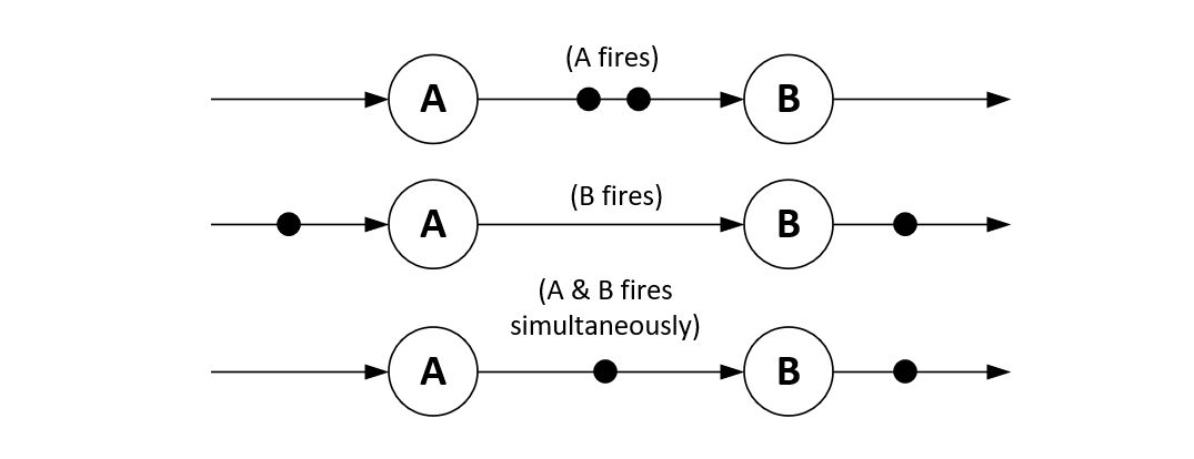
Marking: The distribution of tokens over a graph of actors and queues is called a
marking. The three possible cases of actor firing (A fires, B fires or A and B fire at the same time) result in three different markings. To an external observer, the marking of a dataflow graph is the only state variable in the systems. Actors are pure functions and do not (or are not allowed to) contain state.
As A and B keep firing according to their firing rule, the final state
of the system will be identical for all cases: there will be two tokens on the output queue of actor B.
Figure: Final state after no more firings possible

Dataflow Schedule: A dataflow schedule is a sequence of actor firings. A schedule in which only one actor fires at a time is called a sequential schedule. A schedule which allows multiple actors to fire concurrently is called a parallel schedule. In the system above, we have discussed three possible schedules from the initial state the the end state.
-
S = {A, B, B}is a sequential schedule which fires firstAand thenBtwo times. -
S = {B, A, B}is a sequential schedule which fires firstB, thenA, and thenBagain. -
S = {(A, B), B}is a parallel schedule which first simultaneously firesAandB, and finally firesB.
Now, to perform computations, tokens are attributed with a value, and the actor functions for A and B are defined. For example, let’s say that A would multiply the input token value by two, and let’s say that B would multiply the input token value by three. And let’s say both initial token values have the value one. We can now compute the token values of the final
system state to be the values ‘3’ and ‘6’.
Figure: Computations in the two-actor system

This final state is reached regardless of the order in
which the actors have fired. As long as each actor follows the firing rule,
the computations in syncrhonous dataflow always obtain the same result.
This is a very important observation, which tells that, regardless of the
execution time of A and B, we will always find the same result.
Synchronous dataflow systems are race-free.
Multi-input Multi-output Actors
Many practical dataflow system work with actors that have more then one input. For example, consider an actor which adds token values together to produce an output token stream. This actor has two inputs, each accepting an input token. The firing rule will fire the actor when a token is present on each input of the actor. The general rule for a synchronous dataflow actor with N inputs is that each of the inputs must hold at least one token. We may similarly create actors with more then one output queue. Each time the actor fires, it will produce a token on each output of the actor. The duplicate actor creates two copies of every input token, one on each of its output queues.
Figure: Two-input add actor and two-output duplicate actor

So we can build graphs with those actors, such as the following accumulator system. As shown, the dataflow system is idle, waiting for a second input token on the add actor. When the second token arrives, the add actor will fire, producing on token on the interconnection queue between the add and duplicate actor. Next, the duplicate actor will fire, producing one output token on the output queue, and a second one on the feedback queue.
Figure: Dataflow accumulator

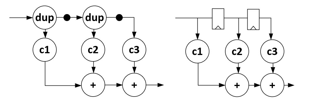
There are several interesting observations to be made. First, a dataflow system with a feedback loop will be deadlocked unless there is at least one token in a queue that defines the loop. Second, if there is only one token in the loop, then only one actor (within that loop) will be able to fire at a time. Hence, the two-actor system shown here will only allow sequential schedules. Third, the token in the feedback loop serves as the ‘storage’ in this system. Neither the add actor nor the duplicate actor contain state; all system state is contained within tokens. You can look at this system with hardware eyes, and imagine a token to be mapped to a register and and the actors to be mapped to combinational logic. Indeed, a synchronous dataflow system has a one-to-one correspondence to a synchronous hardware circuit.
Another example of the one-to-one correspondence between synchronous hardware and synchronous dataflow is this filter design. While the notation is very similar, keep in mind that the semantics of these two models are quite different. The connections in hardware are wires, and they have no storage capability; the connections in synchronous dataflow are queues, and they have infinite storage capability. The nodes in the hardware netlist are blocks of combinational logic. The nodes in the synchronous dataflow graph are actors that use a firing rule.
Figure: Synchronous Dataflow and Synchronous Hardware
Multi-rate Actors and Multi-rate Dataflow
A variant of synchronous dataflow is multi-rate dataflow, which allows more than one token to be consumed or produced per actor firing. The number of tokens consumed per actor firing is called the consumption rate; the number of tokens produced per actor firing is called the production rate. In synchronous dataflow, all production and consumption rates are 1. In multirate dataflow, all production and consumption rates are integer numbers high than or equal to 1.
The following is an example of an multirate system with two actors.
The production and consumption rates are annotated with each input
and each output. Actor A requires two tokens to fire, and will
produce two tokens when it does. Actor B uses only one token
to fire, and produces one token when it does.
This system works according to the following sequential schedule: fires
B fires, then A, then B fires two times, then A again, and so on. We use
the following shorthand notation: S = {B, A, B, B, A, B, B, A, ..} = {B, {A, B, B}+ }. In stead-state, actor B needs to fire twice as much
as actor A, in order to keep up with the token rates produced by A.
Figure: Multi-rate Dataflow

Analysis of multi-rate Dataflow systems
When we run into more complex dataflow systems, it is not obvious what the possible schedules are, which may occur. In the following, we derive a technique to compute a schedule for a multi-rate dataflow system.
First, not all multi-rate dataflow systems result in a
feasible multi-rate schedule. The following are two examples
where such a multi-rate schedule either does not exist, or
else (if it does exist), it results in a non-realizable design.
The graph on the left shows a system that is dead-locked.
Actor B cannot fire because it misses an input token, and a
actor A cannot fire because it does not see sufficient input
tokens. The graph on the left can fire but, each time A runs,
there is an additional token added to the system. Eventually,
the number of tokens in this system will become infinitely
large. While the actors keep on firing, you’d need in finite
amount of storage to hold the value of all tokens produced.
Either of these two cases - deadlock or unbounded token storage - are undesirable. Instead, we want a deadlock-free design, and we want bounded token storage. Furthermore, we want to get a schedule that is periodic, and that can repeat forever. Such a periodic schedule allows unbounded execution of the dataflow system.
Figure: Ill-formed Multi-rate Dataflow

The following technique will demonstrate if a periodic schedule exists. It consists of transforming the dataflow graph into a system of equations that reflect the number of tokens on each queue, and then show that these equations can be solved by a period schedule.
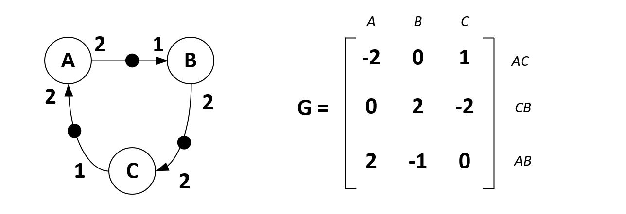
First, we create a topology matrix G. A topology matrix has one row
per queue and one column per actor. The production and consumption
rate are marked as the entries in this matrix, where production rates
are positive and consumption rates are negative. Thus, you can look
at this matrix as describing how the number of tokens in the system
changes as each actor fires.
The followin example shows three actors, A, B and C connected with
three queues. This results in a matrix with three columns (actors) and
three rows (queues) as shown on the right of the figure. The actor
rows and edge columns can be be placed in any order as long as they are
consistently marking the production and consumption rates of the graph.
The number of initial tokens in the graph do not play a role in the
construction of G, even though they will play a role in the eventual
derivation of a concrete sequential or parallel schedule.
Figure: Topology Matrix
The second step is to define the firing vector q, which is the reflects
firings of the three actors. For example a firing vector q = [2 1 1]'
(with ' indicating transpositon) lets A fire two, B fire once, and C fire once. These firings are hypothetical; they ignore if the firing rule
of A, B and C would allow this. The firing vector just says ‘suppose
that we run the actors as follows …’.
Using the firing vector and the topology matric, the number of tokens added
to the system as a result of the firing vector can be computed. For example,
for the firing vector q = [2 1 1]' we find the token vector G.q = [-3 0 3]'. This token vector means that, as a result of executing this firing
vector, three tokens will disappear out of queue AC, three will appear
in queue AB, and none will appear in CB.
         | -2  0  1 |      | 2 |         | -3 |
     G = |  0  2 -2 |  q = | 1 |   G.q = |  0 |
         |  2 -1  0 |      | 1 |         |  3 |
Using the topology matrix and the firing vector, we can show that a periodic admissible schedule exists. A periodic admissible schedule is one that allows unbounded execution and that does not result in deadlock, nor requires infinite queue storage.
We are looking for a firing vector that will keep the amount of tokens in the system stable. In other words, we are looking for a firing vector qn for which the following holds.
G . qn = 0
We also have to show that the system G.qn has an infinite number
of solutions for qn. It’s easy to see what that is needed. If the schedule
is periodic and unbounded, and a given firing vector qn would be a solution, then any multiple k > 0 of this firing vector k.qn must be a solution as well.
The second condition is defined by computing the rank of G. The rank of
a matrix is the number of independent equations in the matrix. If we
have as many equations as there are unknowns (firing rates), then we would
have exactly one solution. However, if we have fewer equations than unknowns, then we have many possible solutions of the form we are looking for. Since the number of unknowns (firing rates) is the same as the number
of actors, we have to show the following:
rank(G) = (number of actors) - 1
In the example system, there are three actors, so we have to show that
the rank of G is two.
                    | -2  0  1 |
     rank(G) = rank(|  0  2 -2 |)
                    |  2 -1  0 |
Since row 2 + 2x (row 1 + row 3) = 0, the three rows in this matrix are not
independent; i.e. we can combine them using scaling, addition and subtraction such that we obtain an all-zero row. We conclude that rank(G)=2.
The next step is to find a solution of G.q = 0. Since we have already
shown that there are an infinite amount of solutions, we only need to find
one.
           | -2  0  1 | |qa|                 | 1 |
     G.q = |  0  2 -2 |.|qb| = 0   <->  qn = | 2 |
           |  2 -1  0 | |qc|                 | 2 |
Thus, in an periodic admissible schedule, actor A will fire twice,
actor B and C will each fire once.
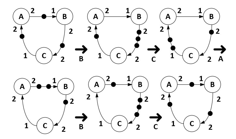
The final step is to derive an actual schedule, which can be done when
we consider the actual dataflow system and the feasible firing vector
qn. Simply try to fire actors iteratively until each actor has reached
the bound indicated in qn. A feasible PASS is the following: S = {B, C, A, B, C}.
Figure: Periodic Admissible Schedule
Applications and Limitations of Dataflow
Dataflow is popular in the modeling of signal processing systems. It’s easy to see why: signal processing systems work with streams of data, and a signal processing chain is often expressed as a chain of modules.
Think about Homework 5, the interpolation filter. This is easy to express as a dataflow system. The UP actor shown below is an upsampling actor, that inserts a zero token for every real value token. This dataflow design can be modeled and simulated, so that the interpolation filter can be verified before implementation in hardware or software.
Figure: Multirate Filter Design in Dataflow
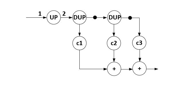
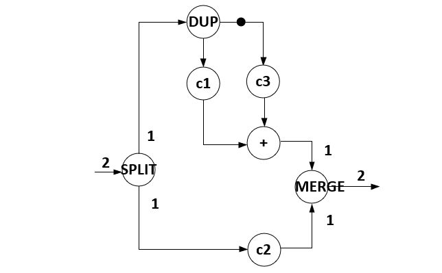
Furthermore, synchronous and multirate dataflow systems
can be transformed and re-analyzed. One popular transformation
is multirate expansion. The interpolation filter shown
above can be broken apart in two pieces, one processing the
odd samples and one processing the even samples. Again,
the result can be captured as a dataflow system, simulated
and verified before the implementation. In the dataflow
system below, the SPLIT and MERGE actors break apart
a sample stream in even and odd samples, and merge it again,
respectively.
Figure: Rate-Expanded Multirate Filter Design in Dataflow
However, synchronous and multirate dataflow modeling is not a universal solution. The weak point of dataflow modeling is that it is unable to express conditional execution. Tokens are produced or consumed, unconditionally. There are many problems that are not easy to capture in dataflow when you are not able to express conditions.
For example, consider doing two possible operations on a token, depending on its value. In C, you capture this easily as follows.
    if (token > 5)
       result = function_one(token);
    else
       result = function_two(token);
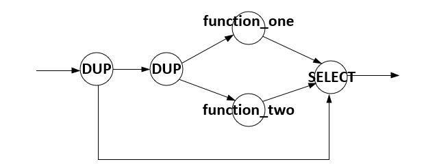
In dataflow, there is no if statement! The best we can do is
execute both function_one and function_two, unconditionally,
and then, depending on the value of the input token, select one
of the two outputs. This can be completely modeling in synchrnous
dataflow as follows.
Figure: Dataflow-if requires computing both true and false case
Further reading on dataflow
-
Dataflow Modeling and Implementation, chapter 2 from “A Practical Introduction to Hardware Software Codesign,” P. Schaumont, Springer 2013.
-
Concurrent Models of Computation, chapter 6 from “Embedded Systems,” E. Lee and S. Seshia, MIT 2017.